Mechanica API Reference¶

This is the API Reference page for the module: mechanica

Simulator¶

class mechanica.Simulator(object)¶

The Simulator is the entry point to simulation, this is the very first object that needs to be initialized before any other method can be called. All the methods of the Simulator are static, but the constructor needs to be called first to initialize everything.

The Simulator manages all of the operating system interface, it manages window creation, end user input events, GPU access, threading, inter-process messaging and so forth. All ‘physical’ modeling concepts to in the Universe object.

__init__(self, conf=None)¶: Initializes a simulation. All of the keyword arguments are the same as on the Config object. You can initialize the simulator via a config Config object , or via keyword arguments. The keywords have the same name as fields on the config.

static run()¶: Starts the operating system messaging event loop for application. This is typically used from scripts, as console input will no longer work. The run method will continue to run until all of the windows are closed, or the quit method is called. By default, run will automatically start the universe time propagation.

static irun()¶: Runs the simulator in interactive mode, in that in interactive mode, the console is still active and users can continue to issue commands via the ipython console. By default, irun will automatically start the universe time propagation.

static quit()¶: Terminates the message loop. The message loop is automatically terminated when all the active windows close.

static show()¶: Shows any windows that were specified in the config. This works just like MatPlotLib’s show method. The show method does not start the universe time propagation unlike run and irun.

class Simulator.Config¶: An object that has all the arguments to the simulator,

Event / Message Processing¶

void glfwPollEvents ( void ) This function processes only those events that are already in the event queue and then returns immediately. Processing events will cause the window and input callbacks associated with those events to be called.

On some platforms, a window move, resize or menu operation will cause event processing to block. This is due to how event processing is designed on those platforms. You can use the window refresh callback to redraw the contents of your window when necessary during such operations.

Universe¶

class mechanica.Universe(object)¶

The universe is a top level singleton object, and is automatically initialized when the simulator loads. The universe is a representation of the physical universe that we are simulating, and is the repository for all phyical object representations.

All properties and methods on the universe are static, and you never actually instantiate a universe.

Universe has a variety of properties such as boundary conditions, and stores all the physical objects such as particles, bonds, potentials, etc..

static bind(thing, a, b)¶

kinetic_energy¶

A read-only attribute that returns the total kinetic energy of the system

Type:	double

dt¶

Get the main simulation time step.

Type:	double

time¶: Get the current simulation time

temperature¶

Get / set the universe temperature.

The universe can be run with, or without a thermostat. With a thermostat, getting / setting the temperature changes the temperture that the thermostat will try to keep the universe at. When the universe is run without a thermostat, reading the temperature returns the computed universe temp, but attempting to set the temperature yields an error.

boltzmann_constant¶: Get / set the Boltzmann constant, used to convert average kinetic energy to temperature

particles¶

List of all the particles in the universe. A particle can be removed from the universe using the standard python del syntax

del Universe.particles[23]

Type:	list

dim¶

Get / set the size of the universe, this is a length 3 list of floats. Currently we can only read the size, but want to enable changing universe size.

Type:	Vector3

static start()¶: Starts the universe time evolution, and advanced the universe forward by timesteps in dt. All methods to build and manipulate universe objects are valid whether the universe time evolution is running or stopped.

static stop()¶: Stops the universe time evolution. This essentially freezes the universe, everythign remains the same, except time no longer moves forward.

static step(until=None, dt=None)¶

Performs a single time step dt of the universe if no arguments are given. Optionally runs until until, and can use a different timestep of dt.

Parameters:	until – runs the timestep for this length of time, optional. dt – overrides the existing time step, and uses this value for time stepping, optional.

Potentials¶

A Potential object is a compiled interpolation of a given function. The Universe applies potentials to particles to calculate the net force on them.

For performance reasons, we found that implmenting potentials as interpolations can be much faster than evaluating the function directly.

A potential can be treated just like any python callable object to evaluate it:

>>> pot = m.Potential.lennard_jones_12_6(0.1, 5, 9.5075e-06 , 6.1545e-03, 1.0e-3 )
>>> x = np.linspace(0.1,1,100)
>>> y=[pot(j) for j in x]
>>> plt.plot(x,y, 'r')

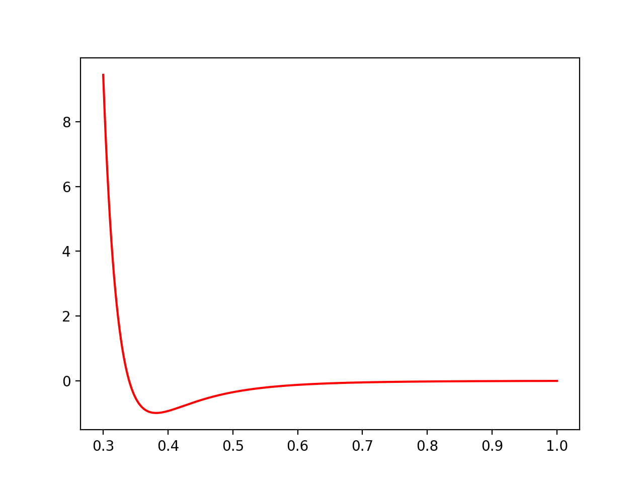
Fig. 16 Potential is a callable object, we can invoke it like any Python function.

class mechanica.Potential¶

static lennard_jones_12_6(min, max, a, b)¶

Creates a Potential representing a 12-6 Lennard-Jones potential

Parameters:	min – The smallest radius for which the potential will be constructed. max – The largest radius for which the potential will be constructed. A – The first parameter of the Lennard-Jones potential. B – The second parameter of the Lennard-Jones potential. tol – The tolerance to which the interpolation should match the exact potential., optional

The Lennard Jones potenntial has the form:

\[\left( \frac{A}{r^{12}} - \frac{B}{r^6} \right)\]

static lennard_jones_12_6_coulomb(min, max, a, b, tol)¶

Creates a Potential representing the sum of a: 12-6 Lennard-Jones potential and a shifted Coulomb potential.

Parameters:

min – The smallest radius for which the potential will be constructed.
max – The largest radius for which the potential will be constructed.
A – The first parameter of the Lennard-Jones potential.
B – The second parameter of the Lennard-Jones potential.
q – The charge scaling of the potential.
tol – The tolerance to which the interpolation should match the exact potential. (optional)

The 12-6 Lennard Jones - Coulomb potential has the form:

\[\left( \frac{A}{r^{12}} - \frac{B}{r^6} \right) + q \left(\frac{1}{r} - \frac{1}{max} \right)\]

static ewald(min, max, q, kappa, tol)¶

Creates a potential representing the real-space part of an Ewald potential.

Parameters:	min – The smallest radius for which the potential will be constructed. max – The largest radius for which the potential will be constructed. q – The charge scaling of the potential. kappa – The screening distance of the Ewald potential. tol – The tolerance to which the interpolation should match the exact potential.

The Ewald potential has the form:

\[q \frac{\mbox{erfc}( \kappa r)}{r}\]

static foo(more stuff)¶

Forces¶

Forces are one of the fundamental processes in Mechanica that cause objects to move. We provide a suite of pre-built forces, and users can create their own.

some stuff here

The forces module collects all of the built-in forces that Mechanica provides. This module contains a variety of functions that all generate a force object.

mechanica.forces.berendsen_thermostat(tau)¶

Creates a Berendsen thermostat

Param:	tau: time constant that determines how rapidly the thermostat effects the system.

The thermostat picks up the target temperature \(T_0\) from the object that it gets bound to. For example, if we bind a temperature to a particle type, then it uses the

The Berendsen thermostat effectively re-scales the velocities of an object in order to make the temperature of that family of objects match a specified temperature.

The Berendsen thermostat force \(\mathbf{F}_{temp}\) has a function form of:

\[\mathbf{F}_{temp} = \frac{\mathbf{p}_i}{\tau_T} \left(\frac{T_0}{T} - 1 \right),\]

where \(T\) is the measured temperature of a family of particles, \(T_0\) is the control temperature, and \(\tau_T\) is the coupling constant. The coupling constant is a measure of the time scale on which the thermostat operates, and has units of time. Smaller values of \(\tau_T\) result in a faster acting thermostat, and larger values result in a slower acting thermostat.

mechanica.forces.dpd_conservative(a, min = 0.1, cutoff=1)¶

Parameters:	a – interaction strength constant min – The smallest radius for which the potential will be constructed. cutoff – The largest radius for which the potential will be constructed. tol – The tolerance to which the interpolation should match the exact

\[\mathbf{F}^C_{ij} = a \left(1 - \frac{r_{ij}}{r_{cutoff}}\right) \mathbf{e}_{ij}\]

mechanica.forces.dpd_dissipative(gamma, min = 0.1, cutoff=1)¶

Parameters:	gamma – interaction strength constant min – The smallest radius for which the potential will be constructed. cutoff – The largest radius for which the potential will be constructed. tol – The tolerance to which the interpolation should match the exact

\[\mathbf{F}^D_{ij} = -\gamma_{ij}\left(1 - \frac{r_{ij}}{r_c}\right)^{0.41}(\mathbf{e}_{ij} \cdot \mathbf{v}_{ij}) \mathbf{e}_{ij}\]

mechanica.forces.dpd_random(gamma, sigma, min, cutoff, tol)¶

Parameters:	gamma – interaction strength constant sigma – standard deviation of the gaussian random noise min – The smallest radius for which the potential will be constructed. cutoff – The largest radius for which the potential will be constructed. tol – The tolerance to which the interpolation should match the exact

\[\mathbf{F}^R_{ij} = \sigma_{ij}\left(1 - \frac{r_{ij}}{r_c}\right)^{0.2} \xi_{ij}\Delta t^{-1/2}\mathbf{e}_{ij}\]