Flux and Transport
Unlike a traditional micro-scale molecular dynamics approach, where each computational particle represents an individual physical atom, a DPD is mesoscopic approach, where each computational particle represents a ‘parcel’ of a real fluid. A single DPD particle typically represents anywhere from a cubic micron to a cubic mm, or about \(3.3 \times 10^{10}\) to \(3.3 \times 10^{19}\) water molecules.
Transport dissipative particle dynamics (tDPD) adds diffusing chemical solutes to each classical DPD particle. Thus, each tDPD particle represents a parcel of bulk fluid (solvent) with a set of chemical solutes at each particle. In tDPD, the main particles represent the bulk medium, or the ‘solvent’, and these carry along, or advect attached solutes. We introduce the term ‘cargo’ to refer to the localized chemical solutes at each particle.
Here we discuss tDPD formalism and demonstrate how to implement a tDPD model using Mechanica.
To attach chemical cargo to a particle, we simply add a Species specifier to
the particle type definition as:
class A(m.Particle):
  species = ['S1', 'S2', S3']
This automatically attaches instance variables S1, S2 and S3 to the
type A, so that every instance of this type has the species attached to
it. Internally Mechanica stores all species in a separate memory block, and the
species symbols are really just accessors. So with the above particle, we can
easily access these values by:
a = A()
a.S1 = 23
print(a.S2)
This simple version of the species keyword defaults to create a set of floating
species, or species who’s value varies in time, and they participate in reaction
and flux processes. We also allow other kinds species such as boundary, or
have initial values, but we refer to these more advanced uses in the
Species section.
Recall that the bulk or solvent particles don’t represent a single molecule, but rather a parcel of fluid. As such, dissolved chemical solutes (cargo) in each parcel of fluid have natural tendency to diffuse to nearby locations.
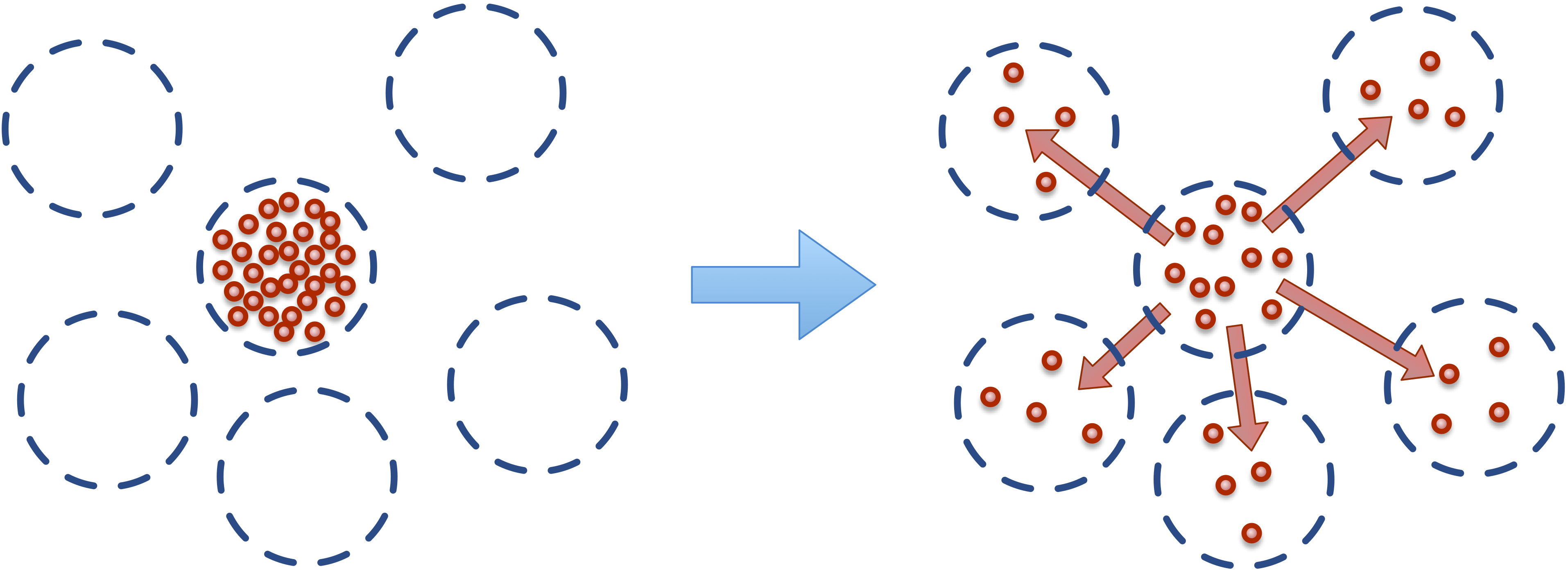
Fig. 11 Dissolved solutes have a natural tendency to diffuse to nearby locations.
This micro-scale diffusion of solutes results in mixing or mass transport without directed bulk motion of the solvent. We refer to the bulk motion, or bulk flow of the solvent as advection, and use convection to describe the combination of both transport phenomena. Diffusion processes are typically either normal or anomalous. Normal (Fickian) diffusion obeys Fick’s laws, and anomalous (non-Fickian) does not.
We introduce the concept of flux to describe this transport of material (chemical solutes) between particles. Fluxes are similar similar to conventional pair-wise forces between particles, in that a flux is between all particles that match a specific type and are within a certain distance from each other. The only differences between a flux and a force, is that a flux is between the chemical cargo on particles, and modifies (transports) chemical cargo between particles, whereas a force modifies the net force acting on each particle.
We attach a flux between chemical cargo as:
class A(m.Particle)
   species = ['S1', 'S2', 'S3']

class B(m.Particle)
   species = ['S1, 'Foo', 'Bar']

q = m.fluxes.fickian(k = 0.5)

m.Universe.bind(q, A.S1, B.S)
m.Universe.bind(q, A.S2, B.Bar)
This creates a Fickian diffusive flux object q, and binds it between species
on two different particle types. Thus, whenever any pair of particles instances
belonging to these types are near each other, the runtime will apply a Fickian
diffusive flux between the species attached to these two particle instances.
In general, the time evolution of the chemical species at each particle are defined by:
where \(Q^D\), \(Q^R\) and \(Q^S\) are the diffusive, random and reactive fluxes. These typically have the form:
where \(\kappa\), \(\epsilon\) are constants, and \(\xi\) is a Gaussian
random number. These fluxes are available in the fluxes.fickian and
fluxes.random packages. We provide more advanced functions, please refer to
the fluxes package for details.
The bulk motion or advection time evolution of a solvent tDPD bulk particle \(i\) obeys both conservation of momentum and mass (solute amount), and is generally written as:
where \(t\), \(\mathbf{r}_i\), \(\mathbf{v}_i\), \(\mathbf{F}\) are time, position velocity, and force vectors, respectively, and \(\mathbf{F}_{ext}\) is the external force on particle \(i\). Forces \(\mathbf{F}^C_{ij}\), \(\mathbf{F}^D_{ij}\) and \(\mathbf{F}^R_{ij}\) are the pairwise conservative, dissipative and random forces respectively.
The conservative force represents the inertial forces in the fluid, and is typically a Lennard-Jones 12-6 type potential. The dissipative, or friction force \(\mathbf{F}^D\) represents the dissipative forces, and the random force \(\mathbf{F}^R\) is a pair-wise random force between particles. Users are of course free to choose any forces they like, but these are the most commonly used DPD ones.
The pairwise forces are commonly expressed as:
Here, \(r_{ij} = |\mathbf{r}_{ij}|\), \(\mathbf{r}_{ij} = \mathbf{r}_i - \mathbf{r}_j\), \(\mathbf{e}_{ij} = \mathbf{r}_{ij} / r_{ij}\). \(\mathbf{v}_{ij} = \mathbf{v}_i - \mathbf{v}_j\).
All of these pairwise forces are conveniently available in the forces package
as the forces.dpd_conservative, forces.dpd_dissipative and
forces.dpd_random respectively.
The parameters in the tDPD system are defined as
- \(\rho = 4.0\)
- \(k_BT=1.0\)
- \(a=75k_B T/ \rho\)
- \(\gamma=4.5\)
- \(\omega^2=2k_B T \gamma\)
- \(r_c=r_{cc} = 1.58\)
- \(\omega_C(r) = (1 - r/r_c)\)
- \(\omega_D(r) = \omega^2_R(r) = (1 -r/r_c)^{0.41}\)
- \(\omega_{DC}(r) = (1 - r/r_{cc})^2\)
and \(\kappa\) ranges from 0 to 10.