Boundary Conditions¶

We can specify a variety of different boundary conditions via the bc argument to the Simulator constructor. We offer a range of boundary condition options in the Boundary Condition Constants section.

We specify boundary conditions via the bc argument to the main init() function call. Boundary conditions can be one of the simple kinds if we use the numeric argument from the Boundary Condition Constants, or can be a dictionary to use flexible boundary conditions.

For flexible boundary conditions, we pass a dictionary to the bc init() argument like:

m.init(bc={'x':'periodic', 'z':'no_slip', 'y' : 'periodic'})

The top-level keys in the bc dictionary can be either "x", "y", "z", or "left", "right", "top", "bottom", "front", or "back". If we choose one of the axis directions, "x", "y", "z", then boundary condition is symmetric, i.e. if we set "x" to some value, then both "left" and "right" get set to that value. Valid options for axis symmetric boundaries are "periodic", "freeslip", "noslip" or "potential".

Note, as a user convenience, we include some synonym, i.e. "no_slip" and "noslip" are equivlent, and "freeslip" and "free_slip" are equivalent.

Periodic¶

The periodic is one of the most widely used boundary condition types in general. This effectively simulates an infinite domain where any agents that leave one side automatically go back in the other. Also, any agents near a boundary will interact with the agents of the opposite boundary, i.e. if there is a repulsive interaction, the agent on the left boundary will be repulsed by an agent on the right boundary. Periodic boundary conditions also determine how chemical fluxes in the Spatial Transport and Flux section operate. With periodic boundaries will, flux will interact with agents on the opposing boundary, but with non-periodic, fluxes will bounce back, or not see any agents on the opposing boundary.

We can specify periodic boundary conditions using either the 'periodic' dictionary argument, or via numeric constants from the Boundary Condition Constants section, i.e.

m.init(bc={'x':'periodic', 'y':'no_slip', 'z' : 'periodic'})

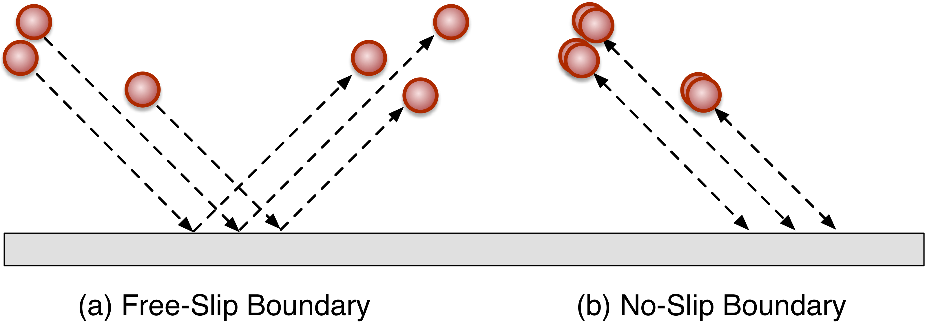
Freeslip and NoSlip¶

Free-slip and no-slip boundary conditions reflect impacting particles back into the simulation domain. Free-slip boundaries are essentially equivalent to a boundary moving at the same tangential velocity with the simulation objects. We can think it as each impacting agent collides with an equivlent ghost agent with the same tangent velocity. No-slip boundaries are equivalent to a stationary wall, in that impacting partricles bounce straight back, inverting their velocity. We can specify these using the 'freeslip' or 'noslip' options to the boundary condition dictionary.

Velocity¶

No-slip boundary conditions are just a specialization of velocity boundaries with zero velocity. Velocity boundaries model a simulation domain with a moving wall boundary. We define a velocity boundary with a nested dictionary to the individual boundary argument, i.e.:

m.init(bc={'top':{'velocity':[-1, 0, 0]},
           'bottom':'noslip',
           'x':'noslip',
           'y':'noslip'})

Potential¶

We can attach a potential to most boundary conditions, and we define a potential only boundary condition using "potential" option, and then bind a potential to the boundary just like we bind potentials between agent types:

m.init(bc={'left':'potential', 'y':'no_slip', 'z' : 'periodic'})
pot = m.Potential.coulomb(q=1, tol=0.0001, min=0.05)
class MyAgent(m.Particle): pass
m.bind(pot, MyAgent, m.universe.boundary_conditions.left)

In this example, we define the left boundary to be a potential type, then add a coulomb potential between that boundary and our agent type, this any instance of that agent will be repulsed by the boundary whenever it is near it.

Potential boundary condtions default to 'free_slip', but we can also create other kinds of potentials, such as say a 'velocity' and bind a potential to that.

Reset¶

The reset boundary condition is a special form of a periodic boundary condition. The basic idea is we have two separate movment processes going on: we have the physical parcels of space (agents) moving around, but they also carry with them a chemical cargo. We have advection (movment of the physical parcels), and diffusion (movment of chemical cargo between agents).

The reset boundary conditions enables us to model driven, advective flow through a domain, where we reset the chemical cargo at the domain boundaries. This is usefull if we model flow where we have chemical sources or sinks in the simulation domain, and do not want any secreted material to re-enter the domain. In effect, this enables us to model an section of domain with driven flow, where the chemical state of the entering flow is always the same.

We enable reset peridic boundaries by setting the boundary condition value to a list of the keywords “periodic” and “reset”, i.e.:

m.init(dt=0.1, dim=[15, 5, 5], cutoff = 3,
     bc={'x':('periodic','reset')})

The reset style boundary condition enables the fluid parcels to pass through periodic boundary conditions normally, howerver it re-sets any attached chemical cargo to the their initially specified values.

A complete example of reset boundary conditons is here with two particles. Here we have two particles, and we can see that the chemical cargo of the moving particle gets reset every time it passes through the periodic domain boundary:

import mechanica as m

m.init(dt=0.1, dim=[15, 5, 5], cutoff = 3,
   bc={'x':('periodic','reset')})

class A(m.Particle):
   species = ['S1', 'S2', 'S3']
   style = {"colormap" : {"species" : "S1",
                         "map" : "rainbow",
                         "range" : "auto"}}

m.flux(A, A, "S1", 2)

a1 = A(m.universe.center - [0, 1, 0])
a2 = A(m.universe.center + [-5, 1, 0], velocity=[0.5, 0, 0])

a1.species.S1 = 3
a2.species.S1 = 0

m.run()