Concepts
Running a Simulation
In most cases, running simulation is as simple as initializing the simulator
with the init function, building the physical model, and calling either the
run or irun methods to run the
simulation. However sometimes users might want more control.
A running simulation has two key components: interacting with the operating
system, and listening for user input, and time stepping the simulation (model)
itself. Whenever the run() or irun() are
invoked, they automatically start time-stepping the simulation. Users can
however explicitly control the time-stepping of the model directly. To display
the window, and start the operating system message loop, you can call the
show() method. This works just like the MatPlotLib show, in that
it displays the windows, but does not time step the simulation. The
Universe.start(), Universe.step(), Universe.stop() methods
start the universe time evolution, perform a single time step, and stop the time
evolution. If the universe is stopped, you can simply call the
Universe.start() method to continue where it was stopped. All methods to build
and manipulate the universe are available either with the universe stopped or
running.
With run(), the function will open the main window, run the simulation, and
will return when the window closes. With irun(), it will open the window,
run the simulation, and return right away, and users can then interact with
simulation objects whilst the simulation is running. Note, only works in the
command line ipython.
For convince, all the the running / showing / closing methods are aliased as top-level methods, i.e.:
>>> import mechanica as m  # import the package
>>> m.init()               # initialize the simulator
>>> # create the model here
>>> ...
>>> m.irun()               # run in interactive mode (only for ipython console)
>>> m.run()                # display the window and run
>>> m.close()              # close the main window
>>> m.show()               # display the window
Building A Model
The first step in formalizing knowledge is writing it down in such a way that it has semantic meaning for both humans and computers. This section will cover the key concepts Mechanica provides that enable users to build models of physical things.
The two key concepts we cover here are objects and processes. Objects are logical representations of physical matter. We use a particle to represent either individual things such as cells, molecules, etc, or particles can represent clumps of matter, such a volume of fluid. Processes are the ways objects interact with each other. Here we will cover the basic interaction potentials that we provide, and will also cover reactions, fluxes and events.
Making Things Move
Newton’s first law states that an object either remains at rest or continues to move at a constant velocity, unless acted upon by a force. That is true regardless if we are considering atoms or galaxies. In order make any object in Mechanica move, we must apply a force to it. To make objects move, Mechanica sums up all of the forces that act on an object, and uses that to calculte the object’s velocity and position.
The nature of forces in Mechanica are incredibly flexible, but we provide a variety of built-in forces to enable common behaviors.
Conservative forces are usually a kind of Potential object, where the
force is described in terms of it’s potential energy function. Long-range,
fluid, and most bonded interactions are examples of conservative potential
energy function based forces. All potential based forces contribute to the total
potential energy of the system, and we can read the total potential energy
either via the Universe.potential_energy attribute, or we can also read
the potential energy of all objects of a type, via the type’s
potential_energy attribute.
We make it easy to create forces, and apply them to objects:
# create a potential, for a simple lennard-jones fluid:
fluid_potential = Potential.lennard-jones-12-6(…)

# bind it to ALL types
m.bind(fluid_potential, Particle, Particle)
This example creates a simple potential, and binds it to ALL objects. As all
objects in our modeling world are either an instance of the base Particle
type, or a instance of a subclass of it.
Coordinate Systems
We can access the cartesian coordinates of any particle via the
Particle.position() method:
>>> p = MyParticleType.items()[0]
>>> print(p.position)
Out[5]: array([8.147237 , 1.3547701, 9.0579195], dtype=float32)
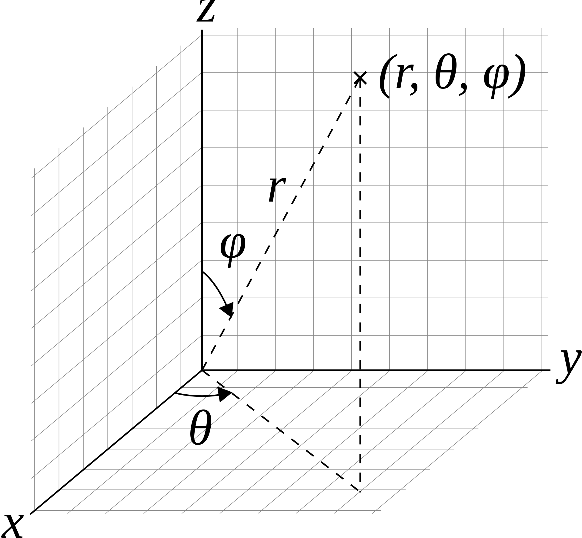
For spherical coordinates, we use the spherical coordinates \((r, \theta, \phi)\) as often used in mathematics: radial distance \(r\), azimuthal angle \(\theta\), and polar angle \(\phi\).
We can get the spherical coordinates of any particle via the
Particle.spherical_position() method, or for a list of partices, we can
call the spherical_positions() method on the list:
>>> In [3]: particles = Cell.items()
>>> In [4]: print(particles.spherical_positions())

    [[11.88918877  1.38879788  0.87157094]
    [13.48884487  1.18363881  1.71954644]
    [13.44023037 -0.2029787   1.40948272]
    ...
    [10.63551331 -1.95453715  1.43269634]
    [13.24325752 -1.98586023  1.21553445]
    [12.08293533 -0.55892485  1.20240927]]
Controlling Temperature
Right now, I have the concept of a ‘Potential’, these are objects that are specified in terms of potential function, and internally, the integrator does a bit of magic with them, and uses them calculate the conservative force that gets added to the total force. Things like bonds, angles, long-range non-bonded forces are all specified in terms of potentials. This works great for conservative forces, and is numerically actually faster then specifying a force function directly. Also, but specifying conservative forces as a potential, that lets me have both a ‘potential_energy’ and a ‘kinetic_energy’ attributes on the universe (and also the object type, i.e. if a user creates a ‘MyParticleType’, they can call MyParticleType.kinetic_energy and this returns the total kinetic energy of all objects of this type).
However, for non-conservative forces, like temperature, friction, etc, these are almost always defined as forces. We can associate a potential energy with a conservative force, but not a non-conservative (or random) force.
That would imply that we need have to allow the user to represent both potentials and forces. I would have preferred to just work in potential or forces, as this simplifies the things for the users, but I don’t really see a way around it.
import mechanica as m
import numpy as np

# potential cutoff distance
cutoff = 1

# dimensions of universe
dim=[10., 10., 10.]

# new simulator
m.init(dim=dim)

# create a potential representing a 12-6 Lennard-Jones potential
# A The first parameter of the Lennard-Jones potential.
# B The second parameter of the Lennard-Jones potential.
# cutoff
pot = m.Potential.lennard_jones_12_6(0.275 , cutoff, 9.5075e-06 , 6.1545e-03 , 1.0e-3 )

# create a particle type
# all new Particle derived types are automatically
# registered with the universe
class A(m.Particle):
    mass = 39.4
    target_temperature = 10000
    radius=0.25

class B(m.Particle):
    mass = 39.4
    target_temperature = 0
    radius=0.25

# bind the potential with the *TYPES* of the particles
m.Universe.bind(pot, A, A)
m.Universe.bind(pot, A, B)
m.Universe.bind(pot, B, B)

# create a thermostat, coupling time constant determines how rapidly the
# thermostat operates, smaller numbers mean thermostat acts more rapidly
tstat = m.forces.berenderson_tstat(10)

# bind it just like any other force
m.Universe.bind(tstat, A)
m.Universe.bind(tstat, B)

size = 10000

# uniform random cube
positions = np.random.uniform(low=0, high=10, size=(size, 6))
velocities = np.random.normal(0, 0.1, size=(size,6))

for (pos,vel) in zip(positions, velocities):
    # calling the particle constructor implicitly adds
    # the particle to the universe
    A(pos[:3], vel[:3])
    A(pos[3:], vel[3:])

# run the simulator interactive
m.Simulator.run()
The complete simulation script is here, and can be downloaded here:
Download: this example script:
So, user experience would be like this:
# create a thermostat force, effectively maintains the temperate of a set of things thermostat = Force.langevin_thermostat(298)
# bind it to all objects of type MyParticle m.bind(thermostat, MyParticle)
# create a friction force friction = Force.friction(…)
# bind it to all objects of type SomeOtherParticle m.bind(friction, SomeOtherParticle)
Binding
Binding objects and processes together is one of the key ways to create a Mechanica simulation. Binding is a very generic concept, but essentially it serves to connect a process (such a potential, flux, reaction, etc..) with one or more objects that that process should act on.
Binding Families of Objects
Binding Individual Objects
Particles
Universe
Collisions / Reactions
Adjective Materials / Diffusive / Dissolved Chemicals
Interacting With The Operating System
The Simulator is manages all of the interaction between the operating
system, end user input, external messaging and the physical model (which resides
in the Universe object.
In order to display a window (s), receive user input, and listen for external
messages, the simulator needs to run an event loop. These are handled by the
Simulator.run() and Simulator.irun() methods.