Potentials and Effect On Mechanics
One of the main goals of Mechanica is to enable users to rapidly develop and explore empirical or phenomenological models of active and biological matter in the 100nm to multiple cm range. There are no pre-defined force fields in this length scale, as such users need a good deal of flexibility to create and calibrate potential functions to model material rheology and particle interactions.
Mechanica provides a wide range of potentials in the Potential class, we can create any of these potential objects using the static methods in this class.
Creating, Plotting and Exploring Potentials
We create a potential object simply by calling one of the static methods on the Potential class. Potential objects conveniently have a plot method on them that displays a ‘matplotlib’ plot, for example:
p = m.Potential.glj(10)
p.plot()
results in
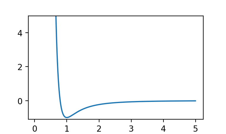
Out:
<Potential at 0x7fb7f6110210>
The Generalized Lennard-Jones Potential, Potential.glj is one of the
most potential we offer, and supports a wide range of parameters. The glj
potential has the form
where \(r_e\) is the effective radius, which is automatically computed as the sum of the interacting particle radii.
In most traditional molecular dynamics packages, it is important to specify the
r0 parameter in a potential, however, Mechanica automatically picks up the rest
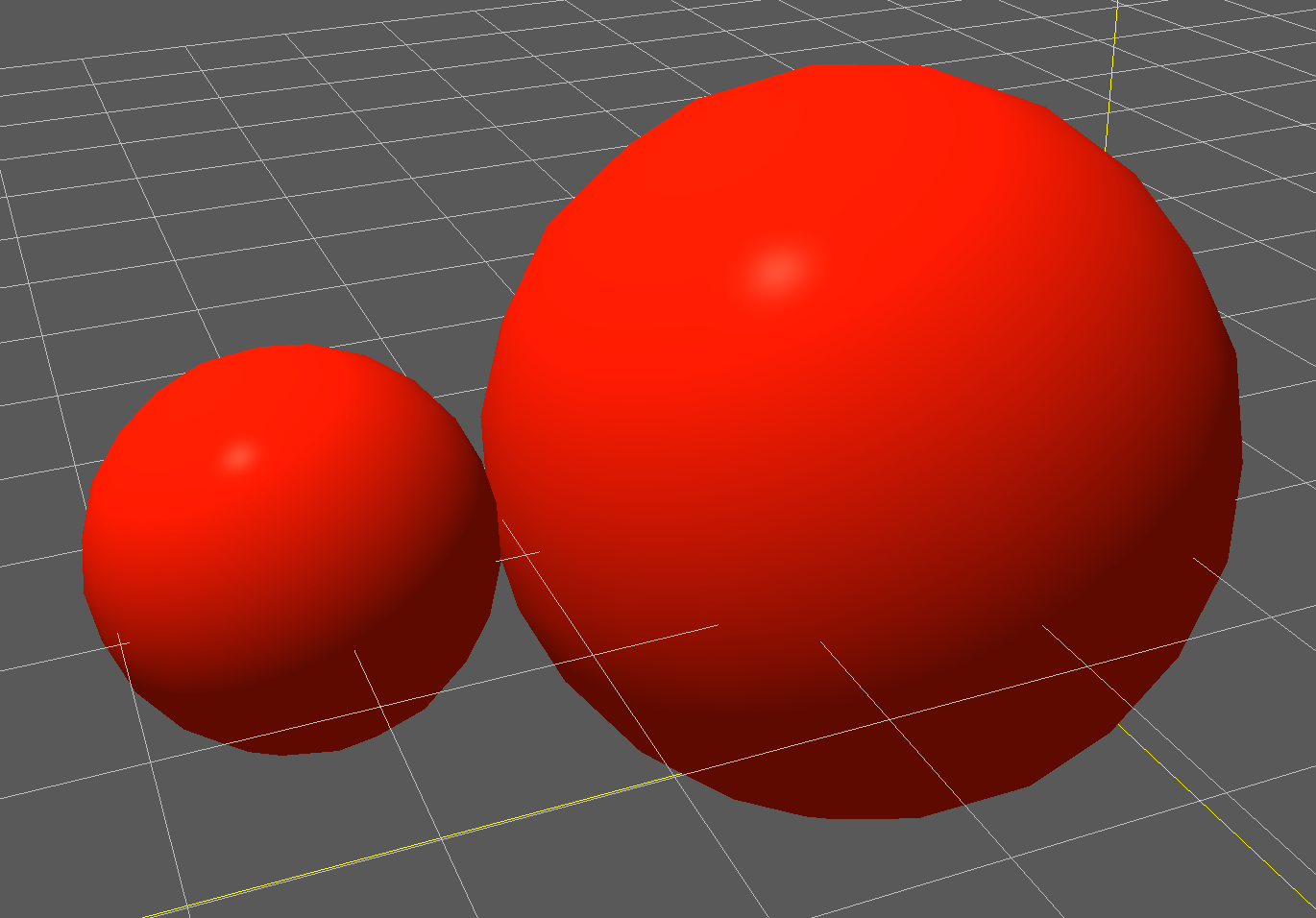
length from the particle radius, For example, say we have two particles, one
with radius 1 and the other with 2, then, if these particles interact with a
potential like glj, they will automatically have a rest separation
distance of 3. We can make a simple model like to illustrate this:
class B(m.Particle):
  mass = 1
  dynamics = m.Overdamped

# make a glj potential, this automatically reads the
# particle radius to determine rest distance.
pot = m.Potential.glj(e=1)

m.bind(pot, B, B)

p1 = B(center + (-2, 0, 0))
p2 = B(center + (2, 0, 0))
p1.radius = 1
p2.radius = 2

m.Simulator.run()
The two particles start out a with a little separation, but the potential pulls them in such that they just touch at the specified radii, and we get an output of:
This complete model is can be downloaded here:
glj-1.py
The Mechanica runtime automatically shifts the potential, such that the minimum of the potential will always be when the separation distance between particles is \(r_1 + r_2\) where \(r_1\) and \(r_2\) are the radii of the two interacting particles.
The most important parameters to glj are the e, r0, m, and min
parameters. The e represents the strength of the potential, it is the depth of
the potential well, and ultimately determines how strongly objects stick
together. r0 is the the lowest point of the potential, and m and n are the
exponents which determine how sharp or shallow the potential is.
e : potential energy
Appropriate values of e should be close to the mass of an object, if e is much larger than about two to three times the mass at most, as this will result in unrealistic behavior and numeric instability. e however can be small as needed to create weakly bound or interacting objects.
r0 : effective radius
The r0 parameter is the effective radius, and determines the equilibrium distance of the potential.
Mechanica however automatically shifts the potential relative to particle radius, so r0 doesn’t determine separation distance as with a traditional molecular dynamics package. Rather r0 influences how soft the potential is. Smaller values of r0 lead to a stiff potential, with a harder shoulder, i.e. it makes the particles harder. Whereas larger values of r0 spread the potential well out over a larger distance, and also allows the potential to be longer ranging, and attract objects from longer distances, as in (A) of Fig. 12.
m : potential exponent
The m and n parameter are the exponents of the potential, and these are principally responsible for how soft or hard the potential is. Small values of m results in a softer, potential, and also allow a longer ranging potential, much like the r0 parameter. It is normally not required to specify the n parameter, as the potential constructor automatically sets this to \(2 * m\), because this format is widely used in many meso-scale particle dynamics based simulations, and results in well-behaved numerics and realistic physical behavior.
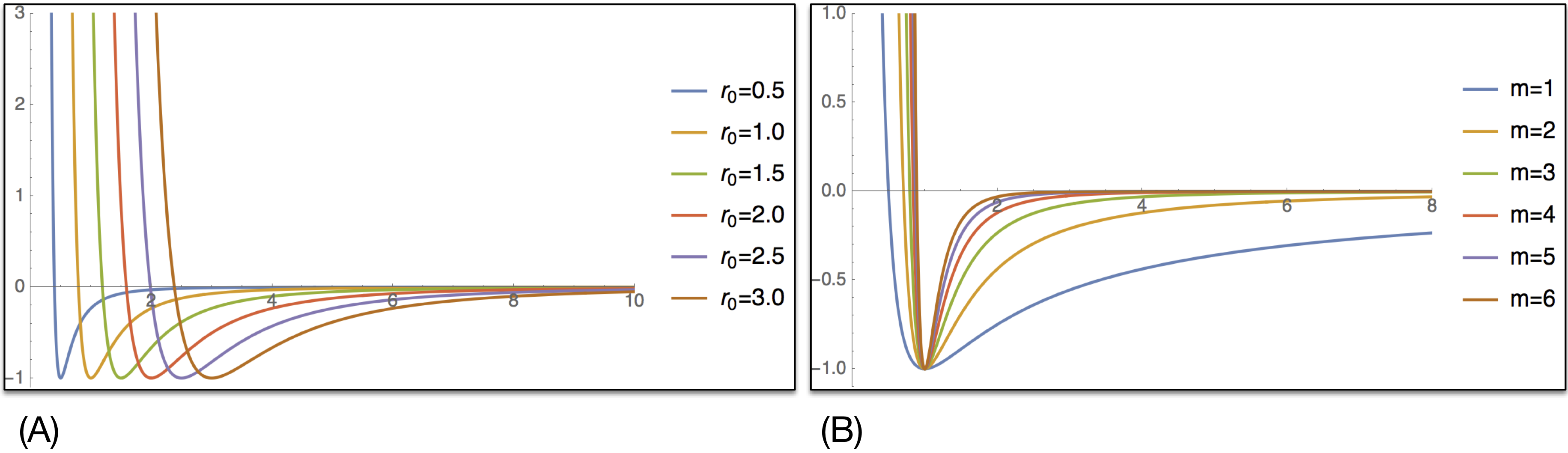
Fig. 12 (A) Varying the \(r_0\) parameter in a glj potential, while holding all other parameters constant, with e=1, m=3, n=6. (B) Varying the m parameter in a glj potential, holding e=1, \(r_0=1\) and with m=2n.
max : potential cutoff distance
The potential cutoff distance, max has a very strong influence on material properties and dynamics. Longer cutoff distances enable us to model things such as an membrane pulling longer distance particles inwards, or long-range coulomb or magnetic potentials, or possibly some more phenomenological interactions such as boids, however longer ranged potentials are typically not very realistic in mesoscopic materials.
In mesoscopic and biological materials, we typically have an interaction that has a short range repulsion – that keeps things from being pushed together, and also a short-range attraction that allows object near each other to stick together, and also lets us model things like fluids, where they like to stick to each other. If we allow longer-range potentials, such as in Fig. 13, we end up with a situation where the particles that make up an object pull so hard on other particles that it causes the object to collapse down to a point. This is especially true when we use a softer potential that does not provide as much short-range repulsion.
For example, we can construct the model that’s shown in Fig. 13
by creating a Cluster type, adding a few particle types to it, and
creating two different potentials to act on them as:
class C(m.Cluster):
  radius=3

  class A(m.Particle):
      radius=0.5
      dynamics = m.Overdamped
      mass=10
      style={"color":"MediumSeaGreen"}

  class B(m.Particle):
      radius=0.5
      dynamics = m.Overdamped
      mass=10
      style={"color":"skyblue"}

c1 = C(position=center - (3, 0, 0))
c2 = C(position=center + (7, 0, 0))

c1.A(2000)
c2.B(2000)

p1  = m.Potential.glj(e=7, m=1, max=1)
p2  = m.Potential.glj(e=7, m=1, max=2)
m.bind(p1, C.A, C.A, bound=True)
m.bind(p2, C.B, C.B, bound=True)

rforce = m.forces.random(0, 10)
m.bind(rforce, C.A)
m.bind(rforce, C.B)
Here we created two very soft glj potentials, we made them soft because
we used m=1 to set the exponent, as discussed earlier. We set one potential to
a cutoff of 1 (twice the particle radius) and the other to a cutoff of 2 (four
times the particle radius). The longer range potential pulls on many more
particles, and the net attraction of these overcomes the relatively soft short
range repulsion. The complete code to create Fig. 13 can be
downloaded here:
glj-1.py
To overcome the this issue of particle clumps collapsing, or overlapping particles, we recommend cutoff distances of around 2-3 times the smallest particle radius. The max cutoff distance defaults to three times the effective radius, r0, we found that this distance generally works well, so users typically would not need to explicitly set this parameter.
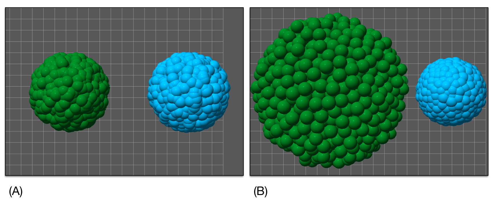
Fig. 13 Two clusters, both with identical particles, and identical initial conditions. The left cluster (green) has a shorter cutoff (twice particle radius), on the potential, ad the right one (blue) has a longer cutoff (four times particle radius). (A) Initializing two clusters of identical particles, both start out the same size. (B) After a few seconds of simulation time, the left