Quickstart
Argon
This example will create a complete simulation of a set of argon atoms.
First we simply import the packages, we will use Numpy to create initial conditions:
import mechanica as m
import numpy as np
Define some variables that define the potential cutoff distance and size of the simulation domain. Potential cutoff is the maximum distance that for which the runtime evaluates potentials, for performance reasons, it should be kept reasonably small
# potential cutoff distance
cutoff = 1

# dimensions of universe
dim=[10., 10., 10.]
The first thing we have to do, before we create any simulation objects is initialize the simulator. This essentially sets up the simulation environment, and gives us a place to create our model.
m.Simulator(dim=dim)
Particles interact via Potentials, Potential. We supply a variety of
pre-built potentials, and users can create their own, but for now, the
Lennard-Jones 12-6 is one of the most commonly used potentials. All we have to
do is create an instance of one, and bind it to an an object type. To create a
LJ potential
# create a potential representing a 12-6 Lennard-Jones potential
# A The first parameter of the Lennard-Jones potential.
# B The second parameter of the Lennard-Jones potential.
# cutoff
pot = m.Potential.lennard_jones_12_6(0.275 , cutoff, 9.5075e-06 , 6.1545e-03 , 1.0e-3 )
It’s most common to sub-class the base particle type. By subclassing it, users can specify a variety of attributes that define that particular type, such as mass.:
# create a particle type
# all new Particle derived types are automatically registered with the universe
class Argon(m.Particle):
    mass = 39.4
Whenever a new Particle derived type is created, it is automatically registerd with the Universe.
The total force on any phyiscal object such as a particle is simply the sum of all potentials that act on that object. To make a potential act on a particular kind of type, we bind the potential to the type of object we want it to act on:
# bind the potential with the *TYPES* of the particles
m.Universe.bind(pot, Argon, Argon)
For our simulation, we want to fill the simulation domain with a uniformly random distrubted particles. The simplest way to do this is the use the numpy random function to generate an array of uniform random distibuted positions:
# uniform random cube
positions = np.random.uniform(low=0, high=10, size=(10000, 3))
Then with the array of positions, we simply itterate over the postions, and create a new particle; When we create a new particle derived object, it gets automatically added to the universe, we don’t need to do anything else with it:
for pos in positions:
    # calling the particle constructor implicitly adds
    # the particle to the universe
    Argon(pos)
Now all that’s left is to run the simulation. The Simulator object has
two methods on it, run and irun. The run method runs the simulator, and
continues until the window is closed, or some stop condition. The irun method
starts the simulation, but leaves the console open for further input. The irun
method is only used when running from iPython.:
# run the simulator interactive
m.Simulator.run()
The complete simulation script is here, and can be downloaded here:
Download: this example script:
import mechanica as m
import numpy as np

# potential cutoff distance
cutoff = 1

# dimensions of universe
dim=[10., 10., 10.]

m.Simulator(dim=dim)

# create a potential representing a 12-6 Lennard-Jones potential
# A The first parameter of the Lennard-Jones potential.
# B The second parameter of the Lennard-Jones potential.
# cutoff
pot = m.Potential.lennard_jones_12_6(0.275 , cutoff, 9.5075e-06 , 6.1545e-03 , 1.0e-3 )

# create a particle type
# all new Particle derived types are automatically
# registered with the universe
class Argon(m.Particle):
    mass = 39.4

# bind the potential with the *TYPES* of the particles
m.Universe.bind(pot, Argon, Argon)

# uniform random cube
positions = np.random.uniform(low=0, high=10, size=(10000, 3))

for pos in positions:
    # calling the particle constructor implicitly adds
    # the particle to the universe
    Argon(pos)

# run the simulator interactive
m.Simulator.run()
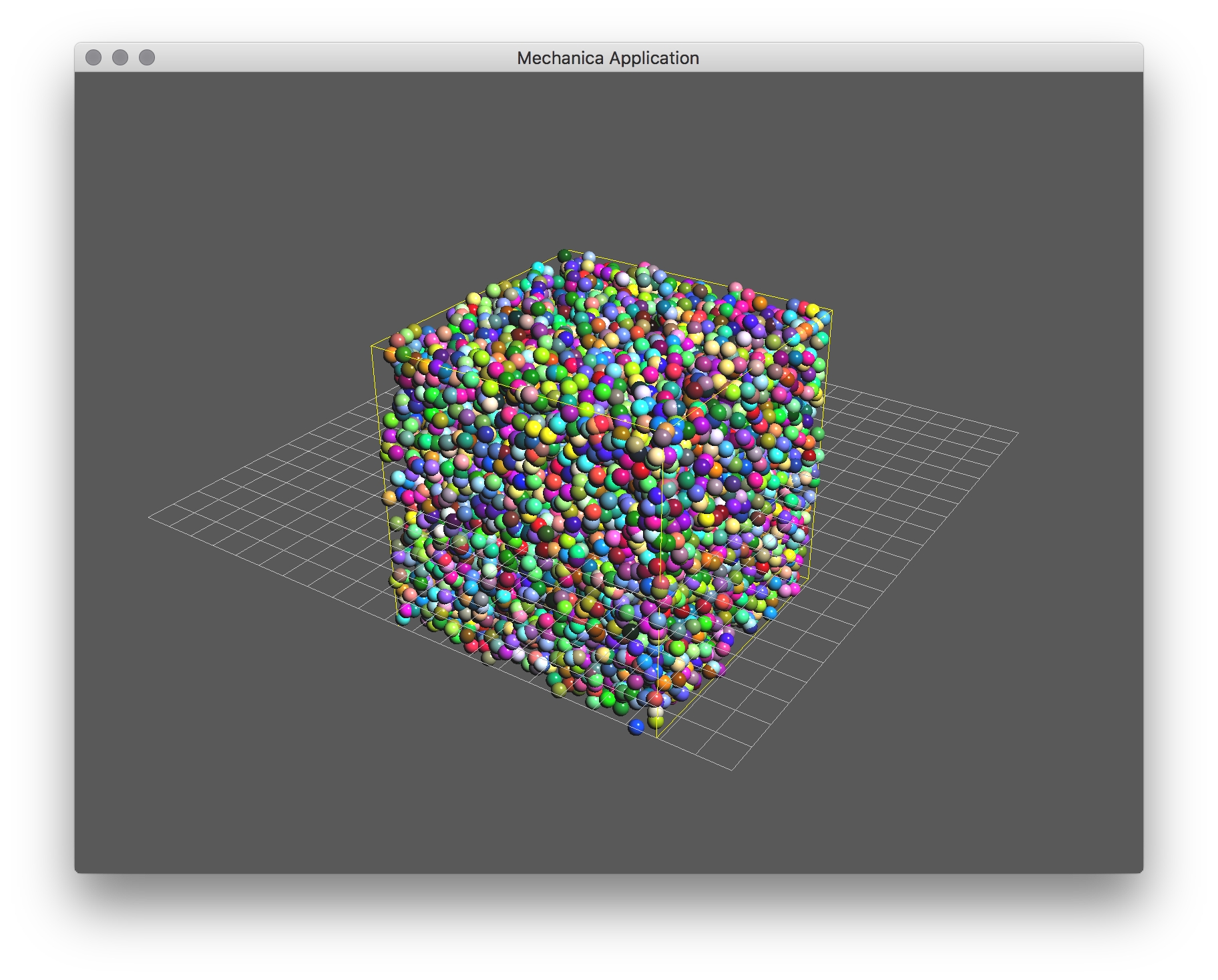
Fig. 3 A basic argon simulation