Chemical Reactions, Flux and Transport
Unlike a traditional micro-scale molecular dynamics approach, where each computational particle represents an individual physical atom, a DPD is mesoscopic approach, where each computational particle represents a ‘parcel’ of a real fluid. A single DPD particle typically represents anywhere from a cubic micron to a cubic mm, or about \(3.3 \times 10^{10}\) to \(3.3 \times 10^{19}\) water molecules.
Transport dissipative particle dynamics (tDPD) adds diffusing chemical solutes to each classical DPD particle. Thus, each tDPD particle represents a parcel of bulk fluid (solvent) with a set of chemical solutes at each particle. In tDPD, the main particles represent the bulk medium, or the ‘solvent’, and these carry along, or advect attached solutes. We introduce the term ‘cargo’ to refer to the localized chemical solutes at each particle.
In general, the time evolution of the chemical species at each spatial object is given as:
where the rate of change of the vector of chemical species at an object is equal to the flux vector, \(Q_i\). This is the sum of the transport and reactive fluxes. \(Q^T\), is the transport flux, and \(Q^R_i\) is a local reactive flux, in the form of a local reaction network. We will cover local reaction fluxes in later paper, for now we restrict this discussion to the passive or ‘Fickian’ flux, secretion flux and uptake flux.
Before we cover spatial transport, we first cover adding chemical reaction networks to objects.
To attach chemical cargo to a particle, we simply add a species specifier to
the particle type definition as:
class A(m.Particle):
  species = ['S1', 'S2', S3']
This defines the three chemical species, S1, S2, and S3 in the type
definition. Thus, when we create an instance of the object, that instance will
have a vector of chemical species attached to it, and is accessible via the
Particle.species attribute. Internally, we allocate a memory block for
each object instance, and users can attach a set of reactions to define the time
evolution of these attached chemical species.
If we access this species list from the type, we get:
>>> print(A.species)
SpeciesList(['S1', 'S2', 'S3'])
This is a special list of SBML species definitions. It’s important to note that once we’ve defined the list of species in each time, that list is immutable. Creating a list of species with just their names is the simplest example, if we need more control, we can create a list from more complex species definition strings in Species.
If a type is defined with a species definition, every instance of that type will get a StateVector, of these substances. Internally, a state vector is really just a contiguous block of numbers, and we can attach a reaction network or rate rules to define their time evolution.
Each instance of a type with a species identifier gets a species attribute, and we can access the values here. In the instance, the species attribute acts a bit like an array, in that we can get it’s length, and use numeric indices to read values:
>>> a = A()
>>> print(a.species)
StateVector([S1:0, S2:0, S3:0])
As we can see, the state vector is array like, but in addition to the numerical values of the species, it contains a lot of meta-data of the species definitions. We can access individual values using array indexing as:
>>> print(a.species[0])
0.0

>>> a.species[0] = 1
>>> print(a.species[0])
1.0
The state vector also automatically gets accessors for each of the species names, and we can access them just like standard Python attributes:
>>> print(a.species.S1)
1.0

>>> a.species.S1 = 5
>>> print(a.species.S1)
5.0
We can even get all of the original species attributes directly from the instance state vector like:
>>> print(a.species[1].id)
'S2'
>>> print(a.species.S2.id)
'S2'
In most cases, when we access the species values, we are accessing the concentration value. See the SBML documentation, but the basic idea is that we internally work with amounts, but each of these species exists in a physical region of space (remember, a particle defines a region of space), so the value we return in the amount divided by the volume of the object that the species is in. Sometimes we want to work with amounts, or we explicitly want to work with concentrations. As such, we can access these with the amount or conc attributes on the state vector objects as such:
>>> print(a.species.amount)
1.0

>>> print(a.species.conc)
0.5
Species
This simple version of the species definition defaults to create a set of floating species, or species who’s value varies in time, and they participate in reaction and flux processes. We also allow other kinds species such as boundary, or have initial values.
The Mechanica Species object is essentially a Python binding around the libSBML Species class, but provides some Pythonic conveniences. For example, in our binding, we use convential Python snake_case sytax, and all of the sbml properties are avialable via simple properties on the objects. Many SBML concepts such as initial_amount, constant, etc. are optional values that may or may not be set. In the standard libSBML binding, users need to use a variety of isBoundaryConditionSet(), unsetBoundaryCondition(), etc… methods that are a direct python binding to the native C++ API. As a convience to our users, our methods simply return a Python None if the field is not set, otherwise returns the value, i.e. to get an initial amount:
>>> print(a.initial_amount)
None
>>> a.initial_amount = 5.0
This internally updates the libSBML Species object that we use. As such, if the user wants to save this sbml, all of these values are set accordingly.
The simplest species object simply takes the name of the species as the only argument:
>>> s = Species("S1")
We can make a boundary species, that is, one that acts like a boundary condition with a “$” in the argument as:
>>> bs = Species("$S1")
>>> print(bs.id)
'S1'
>>> print(bs.boundary)
True
The Species constructor also supports initial values, we specify these by adding a “= value” right hand side expression to the species string:
>>> ia = Species("S1 = 1.2345")
>>> print(ia.id)
'S1'
>>> print(ia.initial_amount)
1.2345
Spatial Transport and Flux
Recall that the bulk or solvent particles don’t represent a single molecule, but rather a parcel of fluid. As such, dissolved chemical solutes (cargo) in each parcel of fluid have natural tendency to diffuse to nearby locations.
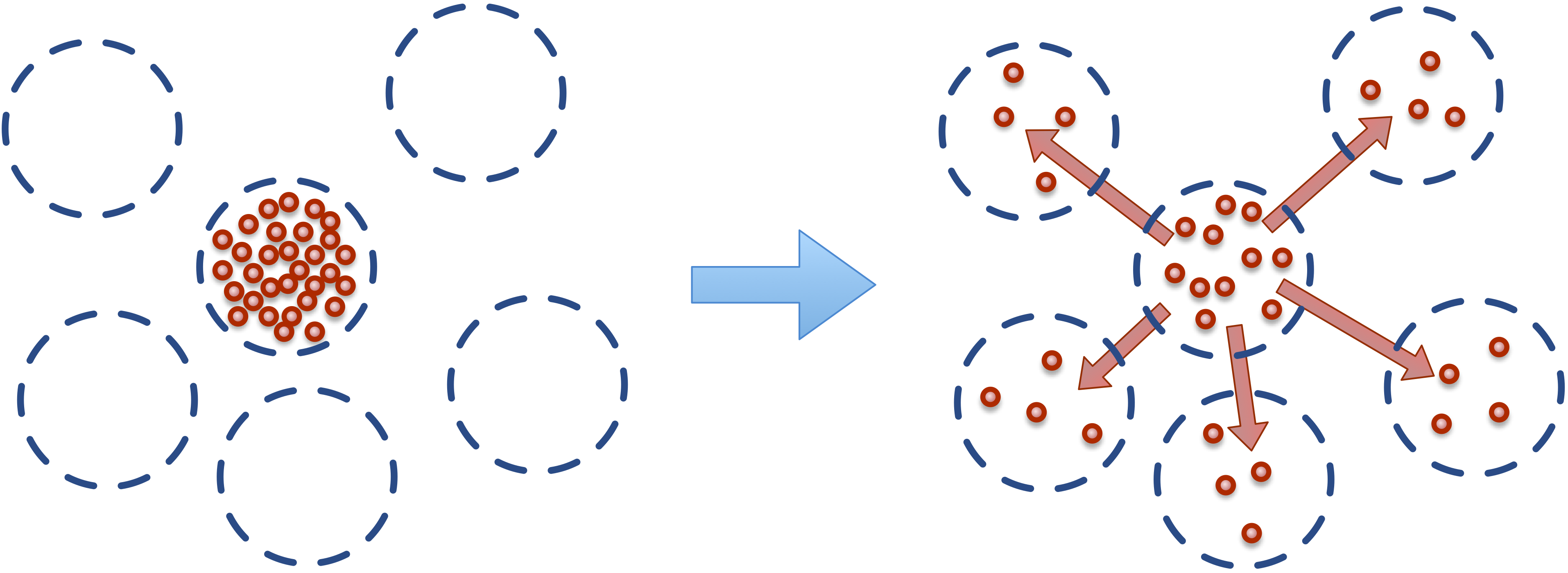
Fig. 15 Dissolved solutes have a natural tendency to diffuse to nearby locations.
This micro-scale diffusion of solutes results in mixing or mass transport without directed bulk motion of the solvent. We refer to the bulk motion, or bulk flow of the solvent as advection, and use convection to describe the combination of both transport phenomena. Diffusion processes are typically either normal or anomalous. Normal (Fickian) diffusion obeys Fick’s laws, and anomalous (non-Fickian) does not.
We introduce the concept of flux to describe this transport of material (chemical solutes) between particles. Fluxes are similar similar to conventional pair-wise forces between particles, in that a flux is between all particles that match a specific type and are within a certain distance from each other. The only differences between a flux and a force, is that a flux is between the chemical cargo on particles, and modifies (transports) chemical cargo between particles, whereas a force modifies the net force acting on each particle.
We attach a flux between chemical cargo as:
class A(m.Particle)
   species = ['S1', 'S2', 'S3']

class B(m.Particle)
   species = ['S1, 'Foo', 'Bar']

q = m.fluxes.fickian(k = 0.5)

m.Universe.bind(q, A.S1, B.S)
m.Universe.bind(q, A.S2, B.Bar)
This creates a Fickian diffusive flux object q, and binds it between species
on two different particle types. Thus, whenever any pair of particles instances
belonging to these types are near each other, the runtime will apply a Fickian
diffusive flux between the species attached to these two particle instances.
Passive Flux: Diffusion
We implement a diffusion process of chemical species located at object instances
using the basic passive (Fickian) flux type, with the flux(). This flux
implements a passive transport between a species located on a pair of nearby objects of type a
and b. A Fick flux of the species \(S\) attached to object types
\(A\) and \(B\) implements the reaction:
\(B\) respectivly. \(S\) is a chemical species located at each object instances. \(k\) is the flux constant, \(r\) is the distance between the two objects, \(r_{cutoff}\) is the global cutoff distance, and \(d\) is the optional decay term.
Active Fluxes: Production and Consumption
For active pumping, to implement such processes like membrane ion pumps, or
other forms of active transport, we provide the produce_flux() and
consume_flux() objects.
The produce flux implements the reaction:
The consumer flux implements the reaction:
Here, the \(\left(1 - \frac{b.S}{b.S_{target}} \right)\) influences the
forward rate, where \([b.S]\) is the concentration of the substance S, and
\(b.S_{target}\) is the target concentration. The flux will continue forward
so long as there is both concentration of the reactant, \(a.S\), and
the product \(b.S\) remains below its target value. Notice that if the
present concentation of \(b.S\) is above its target, the reaction will
proceed in the reverse direction. Thus, the pumping_flux() can be used to
implement both secretion and uptake reactions.