Mechanica API Reference¶

This is the API Reference page for the module: mechanica

mechanica.init(...)¶: Initializes a simulation. All of the keyword arguments are the same as on the Config object. You can initialize the simulator via a config Config object , or via keyword arguments. The keywords have the same name as fields on the config.

mechanica.run()¶: Starts the operating system messaging event loop for application. This is typically used from scripts, as console input will no longer work. The run method will continue to run until all of the windows are closed, or the quit method is called. By default, run will automatically start the universe time propagation.

mechanica.irun()¶: Runs the simulator in interactive mode, in that in interactive mode, the console is still active and users can continue to issue commands via the ipython console. By default, irun will automatically start the universe time propagation.

mechanica.close()¶: Closes the main window, but the application / simulation will continue to run.

mechanica.show()¶

Shows any windows that were specified in the config. This works just like MatPlotLib’s show method. The show method does not start the universe time propagation unlike run and irun.

Keyword Arguments:

dim (vector3 like) – [x,y,z] dimensions of the universe, defaults to [10., 10., 10.]
bc (number or dictionary) – Boundary conditions, use one of the constants in the Boundary Condition Constants section. Defaults to PERIODIC_FULL. For a detailed discussion of boundary condtion options, see Boundary Conditions
cutoff (number) – Cutoff distance for long range forces, try to keep small for best performance, defaults to 1
cells (vector3 like) – [x,y,z] dimensions of spatial cells, how we partition space. Defaults to [4,4,4]
threads (number) – number of compute threads, defaults to 4
integrator (number) – kind of integrator to use, defaults to FORWARD_EULER
dt (number) – time step (\(\delta t\)). If you encounter numerical instability, reduce time step, defaults to 0.01

Simulator¶

mechanica.version(str)¶: The current Mechanica version, as a string.

class mechanica.Simulator(object)¶

The Simulator is the entry point to simulation, this is the very first object that needs to be initialized before any other method can be called. All the methods of the Simulator are static, but the constructor needs to be called first to initialize everything.

The Simulator manages all of the operating system interface, it manages window creation, end user input events, GPU access, threading, inter-process messaging and so forth. All ‘physical’ modeling concepts to in the Universe object.

__init__(self, conf=None, **kwargs)¶: The Simulator(...) construtor call is really just a synonum for the main init() function. We keep this call here as earlier versions used this as the init.

static run()¶: alias to top level mechanica.run() function.

static irun()¶: alias to top level mechanica.irun() function.

static close()¶: alias to top level mechanica.close() function.

static show()¶: alias to top level mechanica.show() function.

class Simulator.Config¶: An object that has all the arguments to the simulator,

Event / Message Processing¶

void glfwPollEvents ( void ) This function processes only those events that are already in the event queue and then returns immediately. Processing events will cause the window and input callbacks associated with those events to be called.

On some platforms, a window move, resize or menu operation will cause event processing to block. This is due to how event processing is designed on those platforms. You can use the window refresh callback to redraw the contents of your window when necessary during such operations.

Universe¶

class mechanica.universe¶

The universe is a top level singleton object, and is automatically initialized when the simulator loads. The universe is a representation of the physical universe that we are simulating, and is the repository for all physical object representations.

All properties and methods on the universe are static, and you never actually instantiate a universe.

Universe has a variety of properties such as boundary conditions, and stores all the physical objects such as particles, bonds, potentials, etc..

static bind(thing, a, b)¶

kinetic_energy¶

A read-only attribute that returns the total kinetic energy of the system

Type:	double

dt¶

Get the main simulation time step.

Type:	double

time¶: Get the current simulation time

temperature¶

Get / set the universe temperature.

The universe can be run with, or without a thermostat. With a thermostat, getting / setting the temperature changes the temperature that the thermostat will try to keep the universe at. When the universe is run without a thermostat, reading the temperature returns the computed universe temp, but attempting to set the temperature yields an error.

boltzmann_constant¶: Get / set the Boltzmann constant, used to convert average kinetic energy to temperature

static particles()¶

List of all the particles in the universe. A particle can be removed from the universe using the standard python del syntax

del universe.particles()[23]

Type:	list

dim¶

Get / set the size of the universe, this is a length 3 list of floats. Currently we can only read the size, but want to enable changing universe size.

Type:	Vector3

static start()¶: Starts the universe time evolution, and advanced the universe forward by timesteps in dt. All methods to build and manipulate universe objects are valid whether the universe time evolution is running or stopped.

static stop()¶: Stops the universe time evolution. This essentially freezes the universe, everything remains the same, except time no longer moves forward.

static step(until=None, dt=None)¶

Performs a single time step dt of the universe if no arguments are given. Optionally runs until until, and can use a different timestep of dt.

Parameters:	until – runs the timestep for this length of time, optional. dt – overrides the existing time step, and uses this value for time stepping, optional.

static grid(shape)¶

Gets a three-dimesional array of particle lists, of all the particles in the system. Each

Parameters:	shape – (length 3 array), list of how many grids we want in the x, y, z directions. Minimum is [1, 1, 1], which will return a array with a single list of all particles.

static virial([origin][, radius][, types])¶

Computes the Virial Tensor for the either the entire simulation domain, or a specific local virial tensor at a location and radius. Optionally can accept a list of particle types to restrict the virial calculation for specify types.

Parameters:	origin – An optional length-3 array for the origin. Defaults to the center of the simulation domain if not given. radius – An optional number specifying the size of the region to compute the virial tensor for. Defaults to the entire simulation domain. types – An optional list of `Particle` types to include in the calculation. Defaults to every particle type.

Boundary Conditions¶

class mechanica.BoundaryCondition¶

name¶: Gets the name of the boundary condition, i.e. “top”, “bottom”, etc..

kind¶: The ‘kind’ of the boundary condition, i.e. “PERIODIC”, “FREESLIP”, or “VELOCITY”

velocity¶: gets / sets the velocity of the boundary, a length-3 vector. Note a “no-slip” boundary is just a “velocity” boundary with a zero velocity vector.

normal¶: get the normal vector of the boundary, points into the simulation domain.

restore¶: gets / sets the restoring percent. When objects hit this boundary, they get reflected back at restore percent, so if restore is 0.5, and object hitting the boundary at 3 length / time recoils with a velocity of 1.5 lengths / time.

class mechanica.Boundaryconditions¶

The BoundaryConditions class really just serves as a contianer for the six instances of the BoundaryCondition object:

left¶

right¶

front¶

back¶

bottom¶

top¶

Boundary Condition Constants¶

mechanica.BOUNDARY_NONE¶: no boundary conditions

mechanica.PERIODIC_X¶: periodic in the x direction

mechanica.PERIODIC_Y¶: periodic in the y direction

mechanica.PERIODIC_Z¶: periodic in the z direction

mechanica.PERIODIC_FULL¶: periodic in all directions

mechanica.PERIODIC_GHOST_X¶

mechanica.PERIODIC_GHOST_Y¶

mechanica.PERIODIC_GHOST_Z¶

mechanica.PERIODIC_GHOST_FULL¶

mechanica.FREESLIP_X¶: free slip in the x direction

mechanica.FREESLIP_Y¶: free slip in the y direction

mechanica.FREESLIP_Z¶: free slip in the z direction

mechanica.FREESLIP_FULL¶: free slip in all directions

Constants¶

Geometry¶

mechanica.Sphere¶

mechanica.SolidSphere¶

mechanica.Disk¶

mechanica.SolidCube¶

mechanica.Cube¶

mechanica.Ring¶

Integrator Constants¶

mechanica.FORWARD_EULER¶: reccomended option, most tested, standard single-step forward Euler

mechanica.RUNGE_KUTTA_4¶: experimental Runge-Kutta-4 integrator.

Particles and Clusters¶

class mechanica.Particle(object)¶

The particle is the most basic physical object we provide. All other physical objects either extend the base Particle, or are collections of particles such as the Cluster

static items()¶: Returns a list of all of the instances of this type.

position¶: vector3 – gets / sets the global position of the particle

velocity¶: vector3 – returns the velocity of the particle, read-only

force¶: vector3 – returns the net force that acts on this particle

charge¶: number – gets the total charge of the particle.

mass¶

radius¶

name¶

name2¶

dynamics¶: number – one of the Integrator Constants that specifies the time evolution of this particle. Particles can be either intertial particles that obey Newtonian dynamics, \(F=ma\) or overdamped dynamics, \(F \propto mv\).

age¶

style¶: Style – gets / sets the style of an object. When we create a new particle instance, it’s style points to the style attribute of the particle’s type, so that if we change something in the particle type, this changes every instance of that type. For more details, see the Style section.

frozen¶: Get / sets the frozen attribute. Frozen particles are fixed in place, and will not move if any force acts on them.

id¶

type_id¶

flags¶

become(type)¶

Dynamically changes the type of an object. We can change the type of a Particle derived object to anyther pre-existing Particle derived type. What this means is that if we have an object of say type A, we can change it to another type, say B, and and all of the forces and processes that acted on objects of type A stip and the forces and processes defined for type B now take over. See section Changing Type for more details.

Parameters:	type – (Type)

split()¶: Splits a single particle into two, for more details, see section Splitting and Cleavage. The particle version of split is fairly simple, however the Cluster.split() offers many more options.

fission()¶: synonym for split()

destroy()¶: Destroys the particle, and removes it form inventory. The present object is handle that now references an empty particle. Calling any method after destroy will result in an error.

spherical([origin])¶

Calculates the particle’s coordinates in spherical coordinates (\([\rho, \theta, \phi]\)), where \(\rho\) is the distance from the origin, \(\theta\) is the azimuthal polar angle ranging from \([0,2 \pi]\), and \(phi\) is the declination from vertical, ranging from \([0,\pi]\)

Parameters:	origin ([x,y,z]) – a vector of the origin to use for spherical coordinate calculations, optional, if not given, uses the center of the simulation domain as the origin.

virial([distance])¶

Computes the virial tensor, see Pressure and Virial Tensors.

Parameters:	distance – (number (,optional)) distance from the center of this particle to include the other particles to use for the virial calculation.
Return type:	3x3 matrix

neighbors([distance][, types])¶

Gets a list of all the other particles that are near the current one. By default, we list all the nearest particles that interact with the current one via forces.

Parameters:

distance – (number (,optional)) - An optional search distance, if specified will get all objects within the given distance. Defaults to the global simulation cutoff distance.
types – (tuple, (,optional)) – If specified, can provide a tuple of types to include in the neighbor search. If types are provides, this method will return all non-cluster particles within a certain distance. Defaults to all types.

For example, to search for all objects of type A and B a distance of 1 unit away from a particle p, we would:

>>> nbrs = p.neighbors(distance=1, types=(A, B))
>>> print(len(nbrs))

class mechanica.Cluster(Particle)¶

A Cluster is a collection of particles.

split([axis][, random][, normal][, point])¶

Splits the cluster into two clusters, where the first one is the original cluster and the new one is a new ‘daughter’ cluster.

split is discussed in detail in Splitting and Cleavage

Parameters:

axis – (length 3 vector (,optional)) - orientation axis for a split. If the ‘axis’ argument is given, the ‘split’ method chooses a random plane co-linear with this vector and uses this as the cleavage plane.
random – (Boolean (,optional)) - ‘split’ chooses a random cleavage plane coincident with the center of mass of the cluster.
normal – (length 3 vector (,optional)) - a normal direction for the cleavage plane.
point – (length 3 vector (,optional)) - if given, uses this point to determine the point-normal form for the clevage plane.

virial()¶: Computes the Virial Tensor for the particles in this cluster.

radius_of_gyration()¶: Computes the Radius of Gyration for the particles in this cluster.

center_of_mass()¶: Computes the Center of Mass for the particles in this cluster.

center_of_geometry()¶: Computes the Center of Geometry for the particles in this cluster.

moment_of_inertia()¶: Computes the Moment of Inertia for the particles in this cluster.

centroid()¶: Convenience synonym for center_of_geometry

inertia()¶: Convenience synonym for moment_of_inertia

ParticleList¶

class mechanica.ParticleList¶

Most Mechanica functions that return a list of particle return a ParticleList. This is a special list type that adds a lot of convenience methods for dealing with spatial information.

virial()¶: Returns the virial, or pressure tensor for all objects in the list.

radius_of_gyration()¶: Computes the radius of gyration

center_of_mass()¶: Computes the center of mass.

center_of_geometry()¶: Computes the center of geometry

centroid()¶: Computes the centroid

moment_of_inertia()¶: Computes the moment of inertia tensor

inertia()¶: Computes the moment of inertia tensor, a synonum for moment_of_intertia()

copy()¶: Creates a deep copy of this list.

positions()¶: Returns a numpy 3xN array of all the particle positions.

spherical_positions([origin])¶: Computes the positions in spherical coordinates relative to an origin, returns a 3xN array.

velocities()¶: Returns a 3xN array of particle velocities

forces()¶: Returns a 3xN array of particle forces.

Potentials¶

A Potential object is a compiled interpolation of a given function. The Universe applies potentials to particles to calculate the net force on them.

For performance reasons, we found that implementing potentials as interpolations can be much faster than evaluating the function directly.

A potential can be treated just like any python callable object to evaluate it:

>>> pot = m.Potential.lennard_jones_12_6(0.1, 5, 9.5075e-06 , 6.1545e-03, 1.0e-3 )
>>> x = np.linspace(0.1,1,100)
>>> y=[pot(j) for j in x]
>>> plt.plot(x,y, 'r')

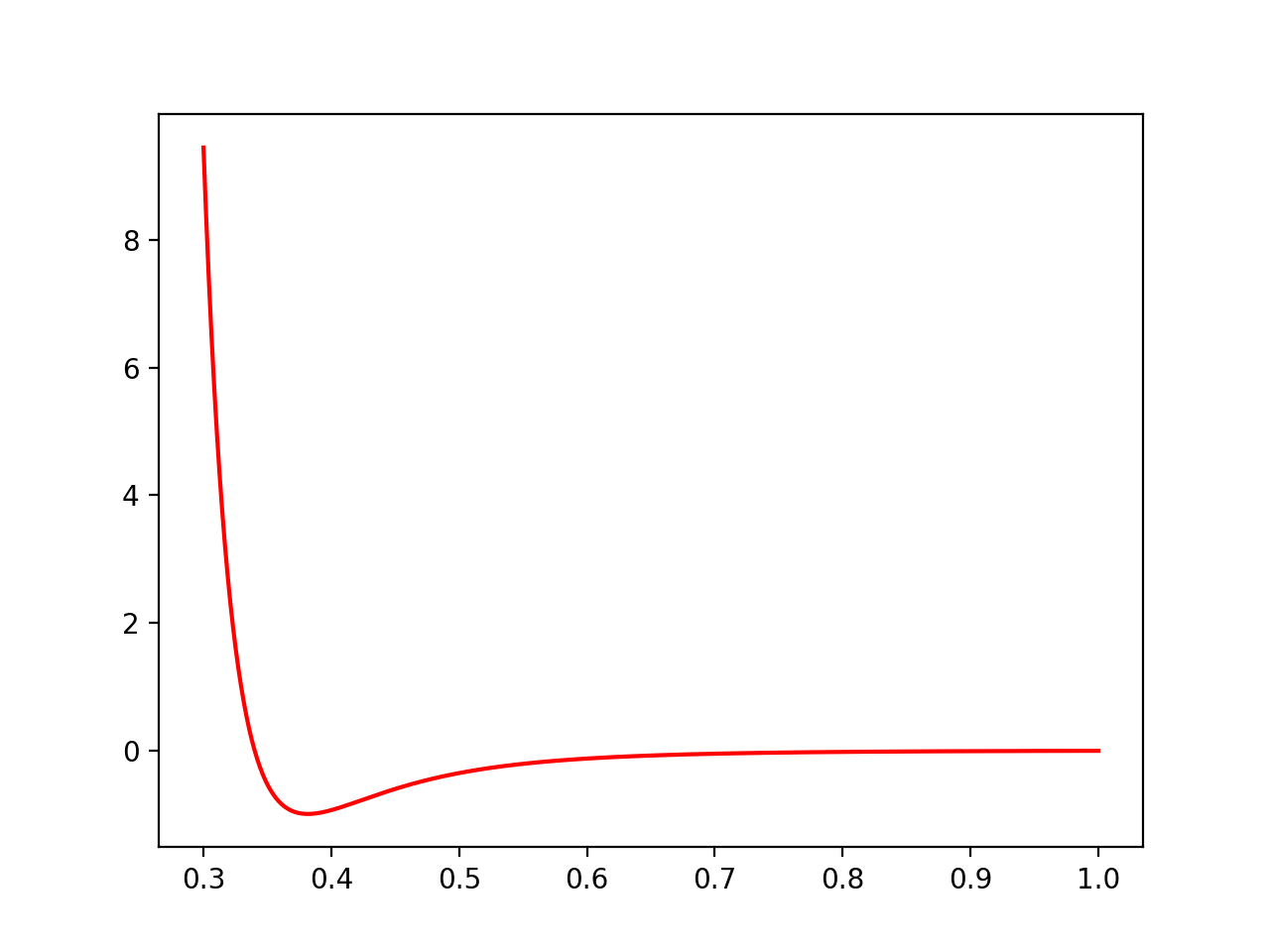
Fig. 20 Potential is a callable object, we can invoke it like any Python function.

class mechanica.Potential¶

static power([k], [r0], [min], max=[10], [tol=0.001])¶
Parameters:

k – interaction strength, represents the potential energy peak value. Defaults to 1

r0 – potential rest length, zero of the potential, defaults to 0.

alpha – Exponent, defaults to 1.

min – minimal value potential is computed for, defaults to r0 / 2.

max – cutoff distance, defaults to 3 * r0.

tol – Tolerance, defaults to 0.01.

some stuff, \(r_0 - r_0 / 2\).

The power potential the general form of many of the potential functions, such as linear(), etc… power has the form:

\[U(r,k) = k (r-r_0)^{\alpha}\]

Some examples of power potentials are:
>>> import mechanica as m
>>> p = m.Potential.power(k=1, r0=1, alpha=1.1)
>>> p.plot(potential=True)
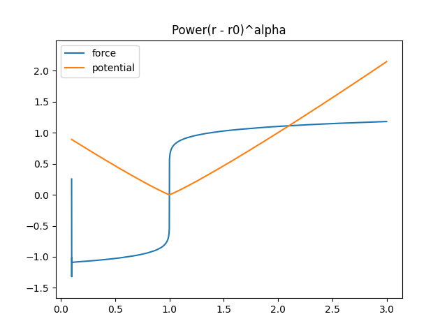
Fig. 21 power potential function of \(U(r) = 1.0 (r - 1)^{1.1}\)
>>> import mechanica as m
>>> p = m.Potential.power(k=1,alpha=0.5, r0=1)
>>> p.plot(potential=True)
Fig. 22 power potential function of \(U(r) = 1.0 (r - 1)^{0.5}\)
>>> import mechanica as m
>>> p = m.Potential.power(k=1,alpha=2.5, r0=1)
>>> p.plot(potential=True)
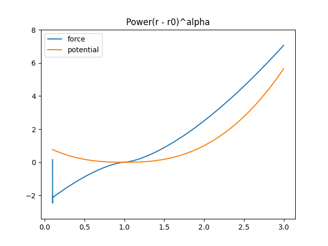
Fig. 23 power potential function of \(U(r) = 1.0 (r - 1)^{2.5}\)

static lennard_jones_12_6(min, max, a, b)¶

Creates a Potential representing a 12-6 Lennard-Jones potential

Parameters:	min – The smallest radius for which the potential will be constructed. max – The largest radius for which the potential will be constructed. A – The first parameter of the Lennard-Jones potential. B – The second parameter of the Lennard-Jones potential. tol – The tolerance to which the interpolation should match the exact potential., optional

The Lennard Jones potential has the form:

\[\left( \frac{A}{r^{12}} - \frac{B}{r^6} \right)\]

static lennard_jones_12_6_coulomb(min, max, a, b, tol)¶

Creates a Potential representing the sum of a: 12-6 Lennard-Jones potential and a shifted Coulomb potential.

Parameters:

min – The smallest radius for which the potential will be constructed.
max – The largest radius for which the potential will be constructed.
A – The first parameter of the Lennard-Jones potential.
B – The second parameter of the Lennard-Jones potential.
q – The charge scaling of the potential.
tol – The tolerance to which the interpolation should match the exact potential. (optional)

The 12-6 Lennard Jones - Coulomb potential has the form:

\[\left( \frac{A}{r^{12}} - \frac{B}{r^6} \right) + q \left(\frac{1}{r} - \frac{1}{max} \right)\]

static ewald(min, max, q, kappa, tol)¶

Creates a potential representing the real-space part of an Ewald potential.

Parameters:	min – The smallest radius for which the potential will be constructed. max – The largest radius for which the potential will be constructed. q – The charge scaling of the potential. kappa – The screening distance of the Ewald potential. tol – The tolerance to which the interpolation should match the exact potential.

The Ewald potential has the form:

\[q \frac{\mbox{erfc}( \kappa r)}{r}\]

static well(k, n, r0[, min][, max][, tol])¶

Creates a continuous square well potential. Usefull for binding a particle to a region.

Parameters:

k (float) – potential prefactor constant, should be decreased for larger n.
n (float) – exponent of the potential, larger n makes a sharper potential.
r0 (float) – The extents of the potential, length units. Represents the maximum extents that a two objects connected with this potential should come appart.
min (float) – [optional] The smallest radius for which the potential will be constructed, defaults to zero.
max (float) – [optional] The largest radius for which the potential will be constructed, defaults to r0.
tol (float) – [optional[ The tolerance to which the interpolation should match the exact potential, defaults to 0.01 * abs(min-max).

\[\frac{k}{\left(r_0 - r\right)^{n}}\]

As with all potentials, we can create one, and plot it like so:

>>> p = m.Potential.well(0.01, 2, 1)
>>> x=n.arange(0, 1, 0.0001)
>>> y = [p(xx) for xx in x]
>>> plt.plot(x, y)
>>> plt.title(r"Continuous Square Well Potential $\frac{0.01}{(1 - r)^{2}}$ \n",
...           fontsize=16, color='black')

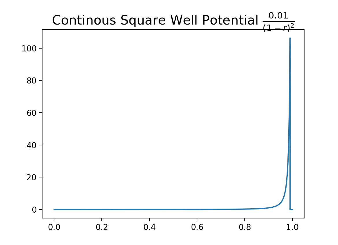
Fig. 24 A continuous square well potential.

static harmonic_angle(k, theta0, [min, ]max[, tol])¶

Creates a harmonic angle potential

Parameters:	k – The energy of the angle. theta0 – The minimum energy angle. min – The smallest angle for which the potential will be constructed. max – The largest angle for which the potential will be constructed. tol – The tolerance to which the interpolation should match the exact potential.

returns A newly-allocated potential representing the potential

\[k(\theta-\theta_0)^2\]

Note, for computational effeciency, this actually generates a function of r, where r is the cosine of the angle (calculated from the dot product of the two vectors. So, this actually evaluates internally,

\[k(\arccos(r)-\theta_0)^2\]

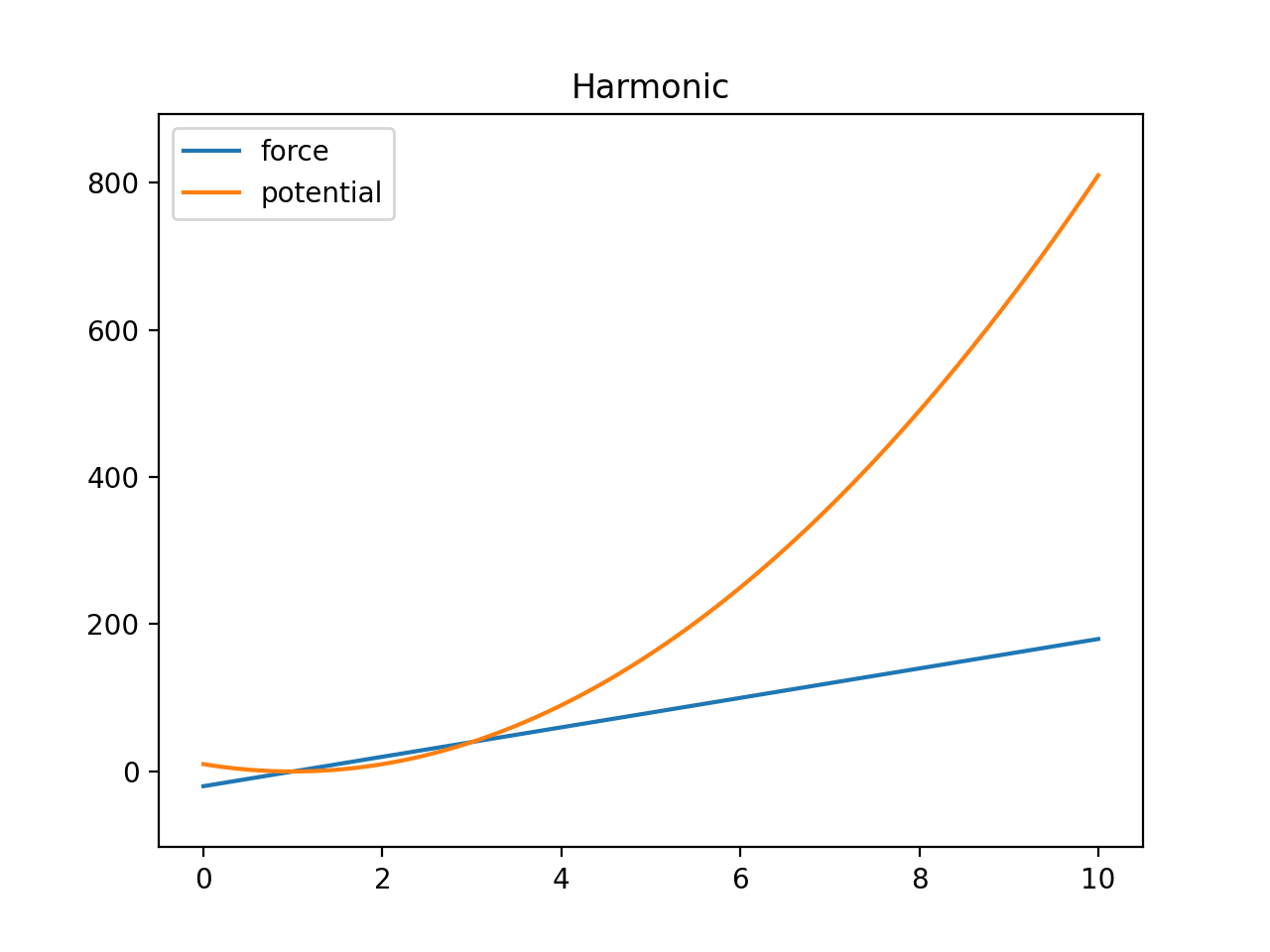
static harmonic(k, r0[, min][, max][, tol])¶

Creates a harmonic bond potential

Parameters:

k – The energy of the bond.
r0 – The bond rest length
min – [optional] The smallest radius for which the potential will be constructed. Defaults to \(r_0 - r_0 / 2\).
max – [optional] The largest radius for which the potential will be constructed. Defaults to \(r_0 + r_0 /2\).
tol – [optional] The tolerance to which the interpolation should match the exact potential. Defaults to \(0.01 \abs(max-min)\)

return A newly-allocated potential

\[U(r) = k (r-r_0)^2\]

We can plot the harmonic function to get an idea of it’s behavior:

>>> import mechanica as m
>>> p = p = m.Potential.harmonic(k=10, r0=1, min=0.001, max=10)
>>> p.plot(s=2, potential=True)

static soft_sphere(kappa, epsilon, r0, eta, min, max, tol)¶

Creates a soft sphere interaction potential. The soft sphere is a generalized Lennard Jones type potentail, but you can varry the exponents to create a softer interaction.

Parameters:	kappa – epsilon – r0 – eta – min – max – tol –

static glj(e[, m][, n][, r0][, min][, max][, tol][, shifted])¶

Parameters:	e – effective energy of the potential m – order of potential, defaults to 3 n – order of potential, defaults to 2m r0 – mimumum of the potential, defaults to 1 min* – minimum distance, defaults to 0.05 * r0 max – max distance, defaults to 5 * r0 tol – tolerance, defaults to 0.01 shifted – is this shifted potential, defaults to true

Generalized Lennard-Jones potential.

\[V^{GLJ}_{m,n}(r) = \frac{\epsilon}{n-m} \left[ m \left( \frac{r_0}{r} \right)^n - n \left( \frac{r_0}{r} \right) ^ m \right]\]

where \(r_e\) is the effective radius, which is automatically computed as the sum of the interacting particle radii.

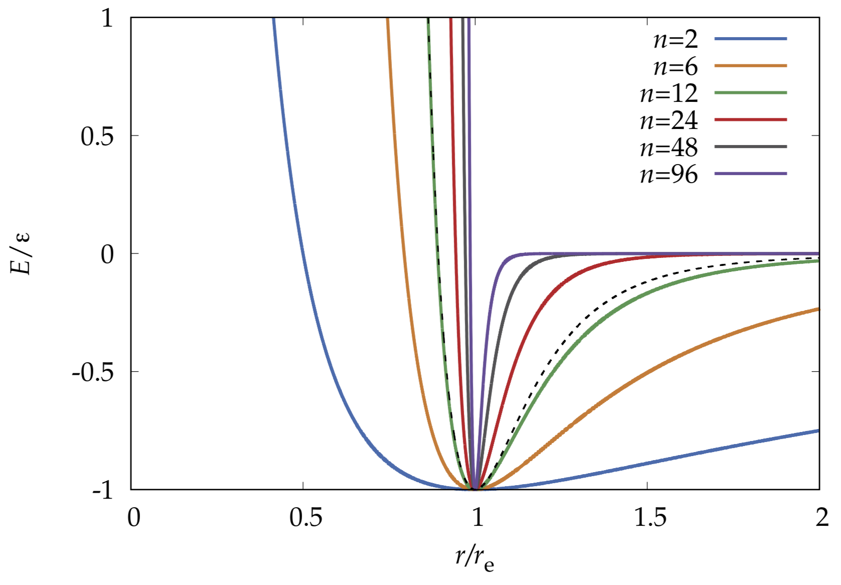
Fig. 25 The Generalized Lennard-Jones potential for different exponents \((m, n)\) with fixed \(n = 2m\). As the exponents grow smaller, the potential flattens out and becomes softer, but as the exponents grow larger the potential becomes narrower and sharper, and approaches the hard sphere potential.

static overlapping_sphere(mu=1, [kc=1], [kh=0], [r0=0], [min=0.001], max=[10], [tol=0.001])¶

Parameters:

mu – interaction strength, represents the potential energy peak value.
kc – decay strength of long range attraction. Larger values make a shorter ranged function.
kh – Optionally add a harmonic long-range attraction, same as glj() function.
r0 – Optional harmonic rest length, only used if kh is non-zero.
min – Minimum value potential is computed for.
max – Potential cutoff values.
tol – Tolerance, defaults to 0.001.

The overlapping_sphere function implements the Overlapping Sphere, from [OFPF+17]. This is a soft sphere, from our testing, it appears too soft, probably better suited for 2D models. This potential appears to allow particles to collapse too closely, probably needs more paramater fiddling.

Note

From the equation below, we can see that there is a \(\log\) term as the short range repulsion term. The logarithm is the radial Green’s function for cylindrical (2D) geometry, however the Green’s function for 3D is the \(1/r\) function. This is possibly why Osborne has success in 2D but it’s unclear if this was used in 3D geometries.

\[\begin{split}\mathbf{F}_{ij}= \begin{cases} \mu_{ij} s_{ij}(t) \hat{\mathbf{r}}_{ij} \log \left( 1 + \frac{||\mathbf{r}_{ij}|| - s_{ij}(t)}{s_{ij}(t)} \right) ,& \text{if } ||\mathbf{r}_{ij}|| < s_{ij}(t) \\ \mu_{ij}\left(||\mathbf{r}_{ij}|| - s_{ij}(t)\right) \hat{\mathbf{r}}_{ij} \exp \left( -k_c \frac{||\mathbf{r}_{ij}|| - s_{ij}(t)}{s_{ij}(t)} \right) ,& \text{if } s_{ij}(t) \leq ||\mathbf{r}_{ij}|| \leq r_{max} \\ 0, & \text{otherwise} \\ \end{cases}\end{split}\]

Osborne refers to \(\mu_{ij}\) as a “spring constant”, this controls the size of the force, and is the potential energy peak value. \(\hat{\mathbf{r}}_{ij}\) is the unit vector from particle \(i\) center to particle \(j\) center, \(k_C\) is a parameter that defines decay of the attractive force. Larger values of \(k_C\) result in a shaper peaked attraction, and thus a shorter ranged force. \(s_{ij}(t)\) is the is the sum of the radii of the two particles.

We can plot the overlapping sphere function to get an idea of it’s behavior:

>>> import mechanica as m
>>> p = m.Potential.overlapping_sphere(mu=10, max=20)
>>> p.plot(s=2, force=True, potential=True, ymin=-10, ymax=8)

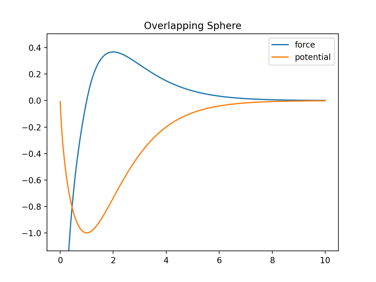
Fig. 26 We can plot the overlapping sphere function like any other function.

static linear(k, [min], max=[10], [tol=0.001])¶

Parameters:	k – interaction strength, represents the potential energy peak value. min – Minimum value potential is computed for. max – Potential cutoff values. tol – Tolerance, defaults to 0.001.

The linear potential is the simplest one, it’s simply a potential of the form

\[U(r) = k r\]

>>> import mechanica as m
>>> p = p = m.Potential.linear(k=5, max=10)
>>> p.plot(potential=True)

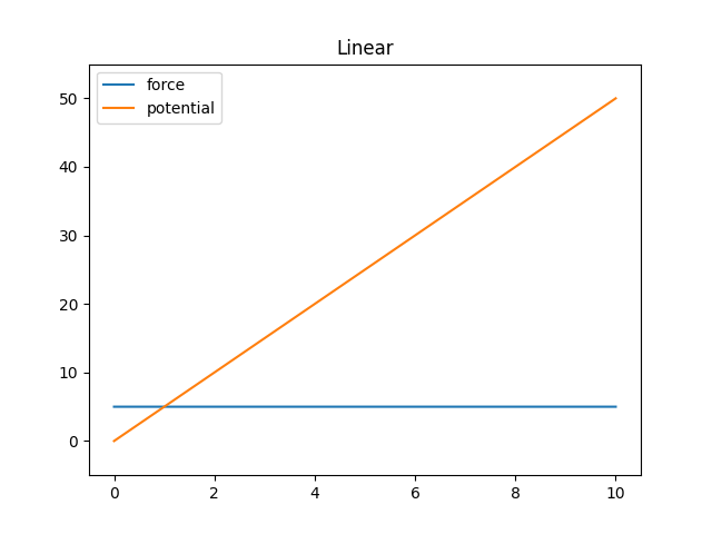
Fig. 27 Linear potential function

Dissapative Particle Dynamics¶

Potential.dpd(alpha=1, gamma=1, sigma=1, cutoff=1)¶

Parameters:	alpha – interaction strength of the conservative force gamma – interaction strength of dissapative force sigma – strength of random force.

The dissapative particle dynamics force is the sum of the conservative, dissapative and random forces:

\[\mathbf{F}_{ij} = \mathbf{F}^C_{ij} + \mathbf{F}^D_{ij} + \mathbf{F}^R_{ij}\]

The conservative force is:

\[\mathbf{F}^C_{ij} = \alpha \left(1 - \frac{r_{ij}}{r_c}\right) \mathbf{e}_{ij}\]

The dissapative force is:

\[\mathbf{F}^D_{ij} = -\gamma \left(1 - \frac{r_{ij}}{r_c}\right)^{2}(\mathbf{e}_{ij} \cdot \mathbf{v}_{ij}) \mathbf{e}_{ij}\]

And the random force is:

\[\mathbf{F}^R_{ij} = \sigma \left(1 - \frac{r_{ij}}{r_c}\right) \xi_{ij}\Delta t^{-1/2}\mathbf{e}_{ij}\]

class mechanica.DPDPotential¶: A subtype of the Potential class that adds features specific to Dissapative Particle Dynamics.

Forces¶

Forces are one of the fundamental processes in Mechanica that cause objects to move. We provide a suite of pre-built forces, and users can create their own.

The forces module collects all of the built-in forces that Mechanica provides. This module contains a variety of functions that all generate a force object.

mechanica.forces.berendsen_thermostat(tau)¶

Creates a Berendsen thermostat

Param:	tau: time constant that determines how rapidly the thermostat effects the system.

The thermostat picks up the target temperature \(T_0\) from the object that it gets bound to. For example, if we bind a temperature to a particle type, then it uses the

The Berendsen thermostat effectively re-scales the velocities of an object in order to make the temperature of that family of objects match a specified temperature.

The Berendsen thermostat force \(\mathbf{F}_{temp}\) has a function form of:

\[\mathbf{F}_{temp} = \frac{\mathbf{p}_i}{\tau_T} \left(\frac{T_0}{T} - 1 \right),\]

where \(T\) is the measured temperature of a family of particles, \(T_0\) is the control temperature, and \(\tau_T\) is the coupling constant. The coupling constant is a measure of the time scale on which the thermostat operates, and has units of time. Smaller values of \(\tau_T\) result in a faster acting thermostat, and larger values result in a slower acting thermostat.

..class:: ConstantForce(value, period=None)

A Constant Force that acts on objects, is a way to specify things like gravity, external pressure, etc…

param value: value can be either a callable that returns a length-3 vector, or a length-3 vector. If value is a vector, than we simply use that vector value as the constant force. If value is callable, then the runtime calls that callable every period to get a new value. If it’s a callable, then it must return somethign convertible to a length-3 array.

param period: If value is a callable, then period defines how frequenly the runtime should call that to obtain a new force value.

Reactions and Species¶

Events are the principle way users can attach connect thier own functions, and built in methods event triggers.

mechanica.on_time(method, period[, start][, end][, distribution])¶

Binds a function or method to a elapsed time interval.

on_time must be called with all keyword arguments, since there are a large number of options this method accepts.

Parameters:

method – A Python function or method that will get called. Signature of the method should be method(time), in that it gets a single current time argument.
period (float) – Time interval that the event should get fired.
start (float) – [optional] Start time for the event.
end (float) – [optional] end time for the event.
distribution (str) – [optional] String that identifies the statistical distribution for event times. Only supported distibution currently is “exponential”. If there is no distibution argument, the event is called deterministically.

Fluxes¶

mechanica.flux(a, b, species_name, k[, decay=0])¶

The basic passive (Fickian) flux type. This flux implements a passive transport between a species located on a pair of nearby objects of type a and b. See Spatial Transport and Flux for a detailed discussion.

Parameters:	a (type) – object type a b (type) – object type b species_name (string) – string, textual name of the species to perform a flux with k (number) – flux rate constant decay (number) – decay rate, optional, defaults to 0.

A Fick flux of the species \(S\) attached to object types \(A\) and \(B\) implements the reaction:

\[\begin{split}\begin{eqnarray} a.S & \leftrightarrow a.S \; &; \; k \left(1 - \frac{r}{r_{cutoff}} \right)\left(a.S - b.S\right) \\ a.S & \rightarrow 0 \; &; \; \frac{d}{2} a.S \\ b.S & \rightarrow 0 \; &; \; \frac{d}{2} b.S, \end{eqnarray}\end{split}\]

\(B\) respectivly. \(S\) is a chemical species located at each object instances. \(k\) is the flux constant, \(r\) is the distance between the two objects, \(r_{cutoff}\) is the global cutoff distance, and \(d\) is the optional decay term.

mechanica.produce_flux(a, b, species_name, k, target[, decay=0])¶

An active flux that represents active transport, and is can be used to model such processes like membrane ion pumps. See Spatial Transport and Flux for a detailed discussion. Unlike the consume_flux, the produce flux uses the concentation of only the source to determine the rate.

Parameters:	a (type) – object type a b (type) – object type b species_name (string) – string, textual name of the species to perform a flux with k (number) – flux rate constant target (number) – target concentation of the \(b.S\) species. decay (number) – decay rate, optional, defaults to 0.

The produce flux implements the reaction:

\[\begin{split}\begin{eqnarray} a.S & \rightarrow b.S \; &; \; k \left(r - \frac{r}{r_{cutoff}} \right)\left(a.S - a.S_{target} \right) \\ a.S & \rightarrow 0 \; &; \; \frac{d}{2} a.S \\ b.S & \rightarrow 0 \; &; \; \frac{d}{2} b.S \end{eqnarray}\end{split}\]

mechanica.consume_flux(a, b, species_name, k, target_concentation[, decay=0])¶

An active flux that represents active transport, and is can be used to model such processes like membrane ion pumps. See Spatial Transport and Flux for a detailed discussion.

Parameters:	a (type) – object type a b (type) – object type b species_name (string) – string, textual name of the species to perform a flux with k (number) – flux rate constant target (number) – target concentation of the \(b.S\) species. decay (number) – decay rate, optional, defaults to 0.

The consume flux implements the reaction:

\[\begin{split}\begin{eqnarray} a.S & \rightarrow b.S \; &; \; k \left(1 - \frac{r}{r_{cutoff}}\right)\left(b.S - b.S_{target} \right)\left(a.S\right) \\ a.S & \rightarrow 0 \; &; \; \frac{d}{2} a.S \\ b.S & \rightarrow 0 \; &; \; \frac{d}{2} b.S \end{eqnarray}\end{split}\]

Bonded Potentials¶

Events¶

Events are the principle way users can attach connect thier own functions, and built in methods event triggers.

mechanica.on_time(method, period[, start][, end][, distribution])

Binds a function or method to a elapsed time interval.

on_time must be called with all keyword arguments, since there are a large number of options this method accepts.

Parameters:

method – A Python function or method that will get called. Signature of the method should be method(time), in that it gets a single current time argument.
period (float) – Time interval that the event should get fired.
start (float) – [optional] Start time for the event.
end (float) – [optional] end time for the event.
distribution (str) – [optional] String that identifies the statistical distribution for event times. Only supported distibution currently is “exponential”. If there is no distibution argument, the event is called deterministically.

mechanica.on_keypress(callback)¶

Register for a key press event. The callback function will get called with a key press object every time the user presses a key. The Keypress object has a key_name property to get the key value:

def my_keypress_handler(e):
    print("key pressed: ", e.key_name)

m.on_keypress(my_keypress_handler)

Style¶

class mechanica.Style(object)¶

The Style object contains all of the rendering visual style attribute of an object. Most simulation objects in Mechanica have a style attribute.

color¶

Color4 – gets / sets the color of the style. This is actually a Color4 object, but we can set it’s color value either as a Color object, or via one of the color strings from Colors, i.e.

>>> c = m.Style()
>>> c.color = "DeepSkyBlue"

The color string is not case sensitive.

visible¶: boolean – gets / sets the visible property. This toggles the visibility of any rendered object.

Colors¶

You can construct a color object, (either a Color3 or Color4) using one of the following web color names:

“AliceBlue”,
“AntiqueWhite”,
“Aqua”,
“Aquamarine”,
“Azure”,
“Beige”,
“Bisque”,
“Black”,
“BlanchedAlmond”,
“Blue”,
“BlueViolet”,
“Brown”,
“BurlyWood”,
“CadetBlue”,
“Chartreuse”,
“Chocolate”,
“Coral”,
“CornflowerBlue”,
“Cornsilk”,
“Crimson”,
“Cyan”,
“DarkBlue”,
“DarkCyan”,
“DarkGoldenRod”,
“DarkGray”,
“DarkGreen”,
“DarkKhaki”,
“DarkMagenta”,
“DarkOliveGreen”,
“Darkorange”,
“DarkOrchid”,
“DarkRed”,
“DarkSalmon”,
“DarkSeaGreen”,
“DarkSlateBlue”,
“DarkSlateGray”,
“DarkTurquoise”,
“DarkViolet”,
“DeepPink”,
“DeepSkyBlue”,
“DimGray”,
“DodgerBlue”,
“FireBrick”,
“FloralWhite”,
“ForestGreen”,
“Fuchsia”,
“Gainsboro”,
“GhostWhite”,
“Gold”,
“GoldenRod”,
“Gray”,
“Green”,
“GreenYellow”,
“HoneyDew”,
“HotPink”,
“IndianRed”,
“Indigo”,
“Ivory”,
“Khaki”,
“Lavender”,
“LavenderBlush”,
“LawnGreen”,
“LemonChiffon”,
“LightBlue”,
“LightCoral”,
“LightCyan”,
“LightGoldenRodYellow”,
“LightGrey”,
“LightGreen”,
“LightPink”,
“LightSalmon”,
“LightSeaGreen”,
“LightSkyBlue”,
“LightSlateGray”,
“LightSteelBlue”,
“LightYellow”,
“Lime”,
“LimeGreen”,
“Linen”,
“Magenta”,
“Maroon”,
“MediumAquaMarine”,
“MediumBlue”,
“MediumOrchid”,
“MediumPurple”,
“MediumSeaGreen”,
“MediumSlateBlue”,
“MediumSpringGreen”,
“MediumTurquoise”,
“MediumVioletRed”,
“MidnightBlue”,
“MintCream”,
“MistyRose”,
“Moccasin”,
“NavajoWhite”,
“Navy”,
“OldLace”,
“Olive”,
“OliveDrab”,
“Orange”,
“OrangeRed”,
“Orchid”,
“PaleGoldenRod”,
“PaleGreen”,
“PaleTurquoise”,
“PaleVioletRed”,
“PapayaWhip”,
“PeachPuff”,
“Peru”,
“Pink”,
“Plum”,
“PowderBlue”,
“Purple”,
“Red”,
“RosyBrown”,
“RoyalBlue”,
“SaddleBrown”,
“Salmon”,
“SandyBrown”,
“SeaGreen”,
“SeaShell”,
“Sienna”,
“Silver”,
“SkyBlue”,
“SlateBlue”,
“SlateGray”,
“Snow”,
“SpringGreen”,
“SteelBlue”,
“Tan”,
“Teal”,
“Thistle”,
“Tomato”,
“Turquoise”,
“Violet”,
“Wheat”,
“White”,
“WhiteSmoke”,
“Yellow”,
“YellowGreen”,

For example, to make some colors::

>>> m.Color3("red")
Vector(1, 0, 0)

>>> m.Color3("MediumSeaGreen")
Vector(0.0451862, 0.450786, 0.165132)

>>> m.Color3("CornflowerBlue")
Vector(0.127438, 0.300544, 0.846873)

>>> m.Color3("this is total garbage")
/usr/local/bin/ipython3:1: Warning: Warning, "this is total garbage" is not a valid color name.
#!/usr/local/opt/python/bin/python3.7
Vector(0, 0, 0)

As it’s easy to make a mistake with color names, we simply issue a warnign, instead of an error if the color name can’t be found.

class mechanica.Color3¶

The class can store either a floating-point or integer representation of a linear RGB color. Colors in sRGB color space should not beused directly in calculations — they should be converted to linear RGB using fromSrgb(), calculation done on the linear representation and then converted back to sRGB using toSrgb().

You can construct a Color object

static from_srgb(srgb(int))¶

constructs a color from a packed integer, i.e.:

>>> c = m.Color3.from_srgb(0xffffff)
>>> print(c)
Vector(1, 1, 1)

Logging¶

Mechanica has extensive logging system. Many internal methods will log extensive details (in full color) to either the clog (typically stderr) or a user specified file path. Internally, the Mechanica logging system is currently implemented by the Poco (http://pocoproject) logging system.

Future versions will include a Logging Listener, so that the Mechanica log will log messages to a user specified function.

The logging system is highly configurable, users have complete control over the color and format of the logging messages.

All methods of the Logger are static, they are available immediately upon loading the Mechanica package.

If one wants to display logging at the lowest level (LOG_TRACE), where every logging message is displayed, one would run:

m.Logging.set_level(m.Logging.LOG_TRACE)

Logging the following messages:

m.Logger.log(m.Logger.LOG_FATAL, "A fatal message")
m.Logger.log(m.Logger.LOG_CRITICAL, "A critical message")
m.Logger.log(m.Logger.LOG_ERROR, "An error message")
m.Logger.log(m.Logger.LOG_WARNING, "A warning message")
m.Logger.log(m.Logger.LOG_NOTICE, "A notice message")
m.Logger.log(m.Logger.LOG_INFORMATION, "An informational message")
m.Logger.log(m.Logger.LOG_DEBUG, "A debugging message.")
m.Logger.log(m.Logger.LOG_TRACE,  "A tracing message. This is the lowest priority.")

will produce the following output:

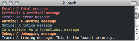
If one wants different colors on the log, these can be set via:

rr.Logger.set_property("traceColor", "red")
rr.Logger.set_property("debugColor", "green")

The available color property names and values are listed below at the Logger.setProperty method.

Logging Levels¶

The Logger has the following logging levels:

Logger.LOG_CURRENT¶: Use the current level – don’t change the level from what it is.

Logger.LOG_FATAL¶: A fatal error. The application will most likely terminate. This is the highest priority.

Logger.LOG_CRITICAL¶: A critical error. The application might not be able to continue running successfully.

Logger.LOG_ERROR¶: An error. An operation did not complete successfully, but the application as a whole is not affected.

Logger.LOG_WARNING¶: A warning. An operation completed with an unexpected result.

Logger.LOG_NOTICE¶: A notice, which is an information with just a higher priority.

Logger.LOG_INFORMATION¶: An informational message, usually denoting the successful completion of an operation.

Logger.LOG_DEBUG¶: A debugging message.

Logger.LOG_TRACE¶: A tracing message. This is the lowest priority.

Logging Methods¶

static Logger.set_level([level])¶

sets the logging level to one a value from Logger::Level

Parameters:	level (int) – the level to set, defaults to LOG_CURRENT if none is specified.

static Logger.get_level()¶: get the current logging level.

static Logger.disable_logging()¶: Suppresses all logging output

static Logger.disable_console_logging()¶: stops logging to the console, but file logging may continue.

static Logger.enable_console_logging(level)¶

turns on console logging (stderr) at the given level.

Parameters:	level – A logging level, one of the above listed LOG_* levels.

static Logger.enable_file_logging(fileName[, level])¶

turns on file logging to the given file as the given level.

Parameters:	fileName (str) – the path of a file to log to. level – (optional) the logging level, defaults to LOG_CURRENT.

static Logger.disable_file_logging()¶: turns off file logging, but has no effect on console logging.

static Logger.get_current_level_as_string()¶: get the textural form of the current logging level.

static Logger.get_filename()¶: get the name of the currently used log file.

static Logger.set_formatting_pattern(format)¶

Internally, Mechanica uses the Poco logging framework, so we can custom format logging output based on a formatting pattern string.

The format pattern is used as a template to format the message and is copied character by character except for the following special characters, which are replaced by the corresponding value.

An example pattern of “%Y-%m-%d %H:%M:%S %p: %t” set via:

m.Logger.set_formatting_pattern("%Y-%m-%d %H:%M:%S %p: %t")

would produce the following output:

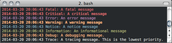
Mechanica supports the following format specifiers. These were copied from the Poco documentation:

%s - message source
%t - message text
%l - message priority level (1 .. 7)
%p - message priority (Fatal, Critical, Error, Warning, Notice, Information, Debug, Trace)
%q - abbreviated message priority (F, C, E, W, N, I, D, T)
%P - message process identifier
%T - message thread name
%I - message thread identifier (numeric)
%N - node or host name
%U - message source file path (empty string if not set)
%u - message source line number (0 if not set)
%w - message date/time abbreviated weekday (Mon, Tue, …)
%W - message date/time full weekday (Monday, Tuesday, …)
%b - message date/time abbreviated month (Jan, Feb, …)
%B - message date/time full month (January, February, …)
%d - message date/time zero-padded day of month (01 .. 31)
%e - message date/time day of month (1 .. 31)
%f - message date/time space-padded day of month ( 1 .. 31)
%m - message date/time zero-padded month (01 .. 12)
%n - message date/time month (1 .. 12)
%o - message date/time space-padded month ( 1 .. 12)
%y - message date/time year without century (70)
%Y - message date/time year with century (1970)
%H - message date/time hour (00 .. 23)
%h - message date/time hour (00 .. 12)
%a - message date/time am/pm
%A - message date/time AM/PM
%M - message date/time minute (00 .. 59)
%S - message date/time second (00 .. 59)
%i - message date/time millisecond (000 .. 999)
%c - message date/time centisecond (0 .. 9)
%F - message date/time fractional seconds/microseconds (000000 - 999999)
%z - time zone differential in ISO 8601 format (Z or +NN.NN)
%Z - time zone differential in RFC format (GMT or +NNNN)
%E - epoch time (UTC, seconds since midnight, January 1, 1970)
%[name] - the value of the message parameter with the given name
%% - percent sign

Parameters:	format (str) – the logging format string. Must be formatted using the above specifiers.

static Logger.get_formatting_pattern()¶: get the currently set formatting pattern.

static Logger.level_to_string(level)¶

gets the textual form of a logging level Enum for a given value.

Parameters:	level (int) – One of the above listed logging levels.

static Logger.string_to_level(s)¶

parses a string and returns a Logger::Level

Parameters:	s (str) – the string to parse.

static Logger.get_colored_output()¶: check if we have colored logging enabled.

static Logger.set_colored_output(b)¶

enable / disable colored output

Parameters:	b (boolean) – turn colored logging on or off

static Logger.set_property(name, value)¶

Set the color of the output logging messages.

In the future, we may add additional properties here.

The following properties are supported:

enableColors: Enable or disable colors.
traceColor: Specify color for trace messages.
debugColor: Specify color for debug messages.
informationColor: Specify color for information messages.
noticeColor: Specify color for notice messages.
warningColor: Specify color for warning messages.
errorColor: Specify color for error messages.
criticalColor: Specify color for critical messages.
fatalColor: Specify color for fatal messages.

The following color values are supported:

default
black
red
green
brown
blue
magenta
cyan
gray
darkgray
lightRed
lightGreen
yellow
lightBlue
lightMagenta
lightCyan
white

Parameters:	name (str) – the name of the value to set. value (str) – the value to set.

static Logger.log(level, msg)¶

logs a message to the log.

Parameters:	level (int) – the level to log at. msg (str) – the message to log.

Rendering and System Interaction¶

The system module contains various function to interact with rendering engine and host cpu.

mechanica.system.cpuinfo()¶: Returns a dictionary that contains a variety of information about the current procssor, such as processor vendor and supported instruction set features.

mechanica.system.gl_info()¶: Returns a dictionary that contains OpenGL capabilities and supported extensions.

mechanica.system.egl_info()¶: Gets a string of EGL info, only valid on Linux, we use EGL for Linux headless rendering.

mechanica.system.image_data()¶: Gets the contents of the rendering frame buffer back as a JPEG image stream, a byte array of the packed JPEG image.

mechanica.system.context_has_current()¶: Checks of the currently executing thread has a rendering context.

mechanica.system.context_make_current()¶: Makes the single Mechanica rendering context current on the current thread. Note, for multi-threaded rendering, the initialization thread needs to release the context via context_release(), then aquire it on the rendering thread via this function.

mechanica.system.context_release()¶: Release the rendering context on the currently executing thread.

mechanica.system.camera_move_to([eye][, center][, up])¶

Moves the camera to the specified ‘eye’ location, where it looks at the ‘center’ with an up vector of ‘up’. All of the parameters are optional, if they are not give, we use the initial default values.

Parameters:	eye – ([x, y, z]) New camera location, where we re-position the eye of the viewer. center – ([x, y, z]) Location that the camera will look at, the what we want as the center of the view. up – ([x, y, z]) Unit up vector, defines the up direction of the camera.

mechanica.system.camera_reset()¶: Resets the camera to the initial position.

mechanica.system.camera_rotate_mouse(mouse_pos)¶

Rotates the camera according to the current mouse position. Need to call camera_init_mouse() to initialize a mouse movement.

Parameters:	mouse_pos – ([x, y]) current mouse position on the view window or image.

mechanica.system.camera_translate_mouse(mouse_pos)¶

Translates the camera according to the current mouse position. You need to call camera_init_mouse() to initialize a mouse movment, i.e. set the starting mouse position.

Parameters:	mouse_pos – ([x, y]) current mouse position on the view window or image.

mechanica.system.camera_init_mouse(mouse_pos)¶

Initialize a mouse movment operation, this tells the simulator that a mouse click was performed at the given coordinates, and subsequent mouse motion will refer to this starting position.

Parameters:	mouse_pos – ([x, y]) current mouse position on the view window or image.

mechanica.system.camera_translate_by(delta)¶

Translates the camera in the plane perpendicular to the view orientation, moves the camera a given delta x, delta y distance in that plane.

Parameters:	delta – ([delta_x, delta_y]) a vector that indicates how much to translate the camera.

mechanica.system.camera_zoom_by(delta)¶

Zooms the camera in and out by a specified amount.

Parameters:	delta – number that indicates how much to increment zoom distance.

mechanica.system.camera_zoom_to(distance)¶

Zooms the camera to the given distance.

Parameters:	distance – distance to the universe center for the camera.

mechanica.system.camera_rotate_to_axis(axis, distance)¶

Rotates the camera to one of the principal axis, at a given zoom distance.

Parameters:	axis – ([x, y, z]) unit vector that defines the axis to move to. distance – how far away the camera will be.

mechanica.system.camera_rotate_to_euler_angle(angles)¶

Rotate the camera to the given orientiation defined by three Euler angles.

Parameters:	angles – ([alpha, beta, gamma]) Euler angles of rotation about the X, Y, and Z axis.

mechanica.system.camera_rotate_by_euler_angle(angles)¶

Incremetns the camera rotation by given orientiation defined by three Euler angles.

Parameters:	angles – ([alpha, beta, gamma]) Euler angles of rotation about the X, Y, and Z axis.

mechanica.system.view_reshape(window_size)¶

Notify the simulator that the window or image size was changed.

Parameters:	window_size – ([x, y]) new window size.