Potentials¶

A Potential object is a compiled interpolation of a given function. The Universe applies potentials to particles to calculate the net force on them.

For performance reasons, we found that implementing potentials as interpolations can be much faster than evaluating the function directly.

A potential can be treated just like any python callable object to evaluate it:

>>> pot = m.Potential.lennard_jones_12_6(0.1, 5, 9.5075e-06 , 6.1545e-03, 1.0e-3 )
>>> x = np.linspace(0.1,1,100)
>>> y=[pot(j) for j in x]
>>> plt.plot(x,y, 'r')

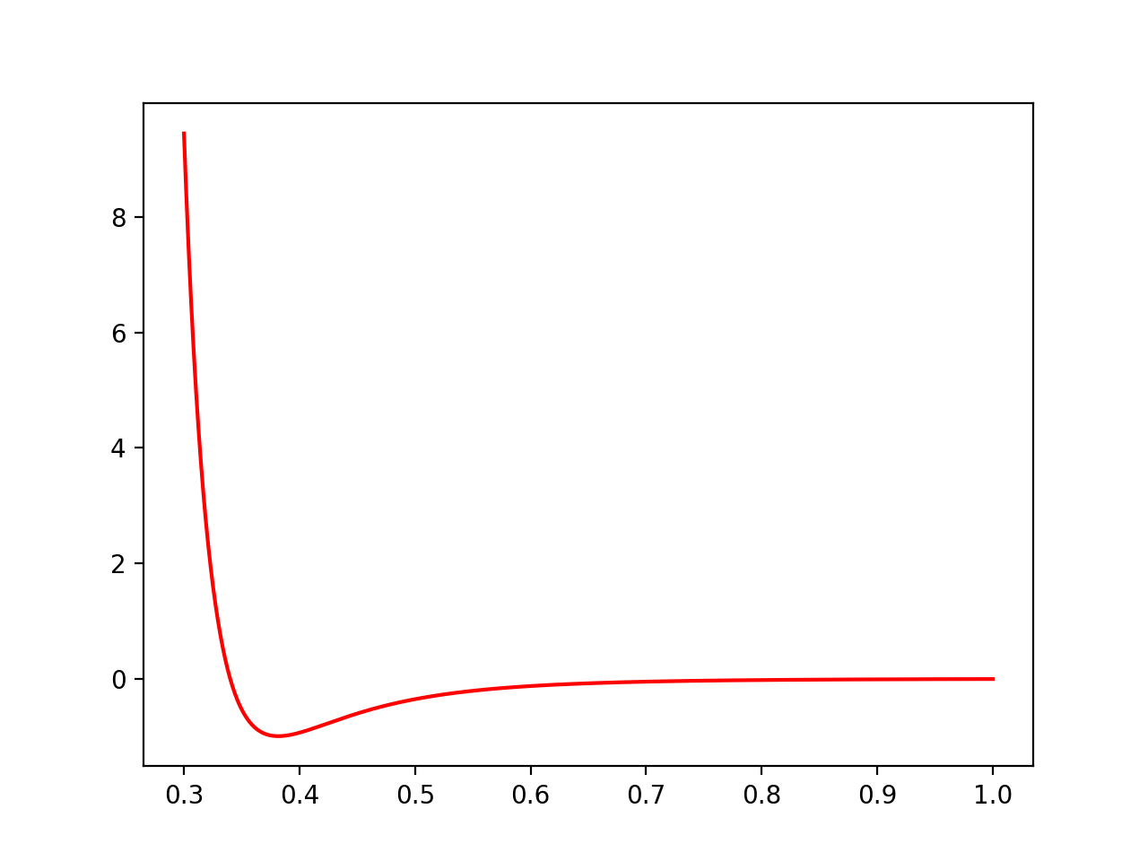
Potential is a callable object, we can invoke it like any Python function.

class Potential¶

static power([k], [r0], [min], max=[10], [tol=0.001])¶
Parameters:

k – interaction strength, represents the potential energy peak value. Defaults to 1

r0 – potential rest length, zero of the potential, defaults to 0.

alpha – Exponent, defaults to 1.

min – minimal value potential is computed for, defaults to r0 / 2.

max – cutoff distance, defaults to 3 * r0.

tol – Tolerance, defaults to 0.01.

some stuff, \(r_0 - r_0 / 2\).

The power potential the general form of many of the potential functions, such as linear(), etc… power has the form:

\[U(r,k) = k (r-r_0)^{\alpha}\]

Some examples of power potentials are:
>>> import mechanica as m
>>> p = m.Potential.power(k=1, r0=1, alpha=1.1)
>>> p.plot(potential=True)
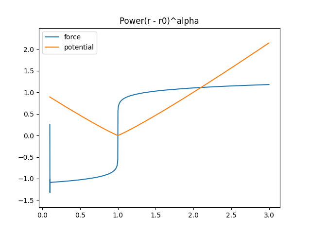
power potential function of \(U(r) = 1.0 (r - 1)^{1.1}\)
>>> import mechanica as m
>>> p = m.Potential.power(k=1,alpha=0.5, r0=1)
>>> p.plot(potential=True)
power potential function of \(U(r) = 1.0 (r - 1)^{0.5}\)
>>> import mechanica as m
>>> p = m.Potential.power(k=1,alpha=2.5, r0=1)
>>> p.plot(potential=True)
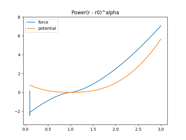
power potential function of \(U(r) = 1.0 (r - 1)^{2.5}\)

static lennard_jones_12_6(min, max, a, b)¶

Creates a Potential representing a 12-6 Lennard-Jones potential

Parameters:	min – The smallest radius for which the potential will be constructed. max – The largest radius for which the potential will be constructed. A – The first parameter of the Lennard-Jones potential. B – The second parameter of the Lennard-Jones potential. tol – The tolerance to which the interpolation should match the exact potential., optional

The Lennard Jones potential has the form:

\[\left( \frac{A}{r^{12}} - \frac{B}{r^6} \right)\]

static lennard_jones_12_6_coulomb(min, max, a, b, tol)¶

Creates a Potential representing the sum of a: 12-6 Lennard-Jones potential and a shifted Coulomb potential.

Parameters:

min – The smallest radius for which the potential will be constructed.
max – The largest radius for which the potential will be constructed.
A – The first parameter of the Lennard-Jones potential.
B – The second parameter of the Lennard-Jones potential.
q – The charge scaling of the potential.
tol – The tolerance to which the interpolation should match the exact potential. (optional)

The 12-6 Lennard Jones - Coulomb potential has the form:

\[\left( \frac{A}{r^{12}} - \frac{B}{r^6} \right) + q \left(\frac{1}{r} - \frac{1}{max} \right)\]

static ewald(min, max, q, kappa, tol)¶

Creates a potential representing the real-space part of an Ewald potential.

Parameters:	min – The smallest radius for which the potential will be constructed. max – The largest radius for which the potential will be constructed. q – The charge scaling of the potential. kappa – The screening distance of the Ewald potential. tol – The tolerance to which the interpolation should match the exact potential.

The Ewald potential has the form:

\[q \frac{\mbox{erfc}( \kappa r)}{r}\]

static well(k, n, r0[, min][, max][, tol])¶

Creates a continuous square well potential. Usefull for binding a particle to a region.

Parameters:

k (float) – potential prefactor constant, should be decreased for larger n.
n (float) – exponent of the potential, larger n makes a sharper potential.
r0 (float) – The extents of the potential, length units. Represents the maximum extents that a two objects connected with this potential should come appart.
min (float) – [optional] The smallest radius for which the potential will be constructed, defaults to zero.
max (float) – [optional] The largest radius for which the potential will be constructed, defaults to r0.
tol (float) – [optional[ The tolerance to which the interpolation should match the exact potential, defaults to 0.01 * abs(min-max).

\[\frac{k}{\left(r_0 - r\right)^{n}}\]

As with all potentials, we can create one, and plot it like so:

>>> p = m.Potential.well(0.01, 2, 1)
>>> x=n.arange(0, 1, 0.0001)
>>> y = [p(xx) for xx in x]
>>> plt.plot(x, y)
>>> plt.title(r"Continuous Square Well Potential $\frac{0.01}{(1 - r)^{2}}$ \n",
...           fontsize=16, color='black')

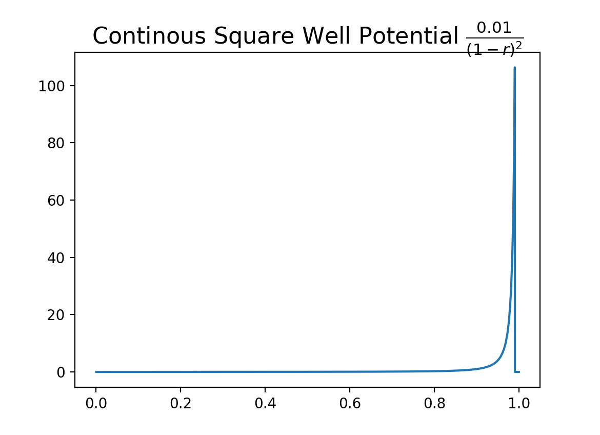
A continuous square well potential.

static harmonic_angle(k, theta0, [min, ]max[, tol])¶

Creates a harmonic angle potential

Parameters:	k – The energy of the angle. theta0 – The minimum energy angle. min – The smallest angle for which the potential will be constructed. max – The largest angle for which the potential will be constructed. tol – The tolerance to which the interpolation should match the exact potential.

returns A newly-allocated potential representing the potential

\[k(\theta-\theta_0)^2\]

Note, for computational effeciency, this actually generates a function of r, where r is the cosine of the angle (calculated from the dot product of the two vectors. So, this actually evaluates internally,

\[k(\arccos(r)-\theta_0)^2\]

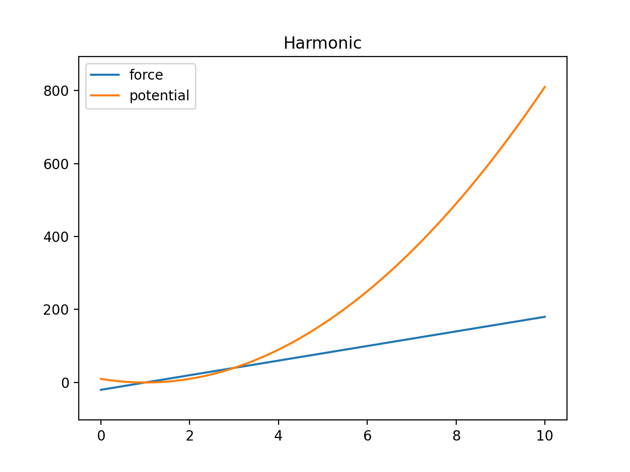
static harmonic(k, r0[, min][, max][, tol])¶

Creates a harmonic bond potential

Parameters:

k – The energy of the bond.
r0 – The bond rest length
min – [optional] The smallest radius for which the potential will be constructed. Defaults to \(r_0 - r_0 / 2\).
max – [optional] The largest radius for which the potential will be constructed. Defaults to \(r_0 + r_0 /2\).
tol – [optional] The tolerance to which the interpolation should match the exact potential. Defaults to \(0.01 \abs(max-min)\)

return A newly-allocated potential

\[U(r) = k (r-r_0)^2\]

We can plot the harmonic function to get an idea of it’s behavior:

>>> import mechanica as m
>>> p = p = m.Potential.harmonic(k=10, r0=1, min=0.001, max=10)
>>> p.plot(s=2, potential=True)

static soft_sphere(kappa, epsilon, r0, eta, min, max, tol)¶

Creates a soft sphere interaction potential. The soft sphere is a generalized Lennard Jones type potentail, but you can varry the exponents to create a softer interaction.

Parameters:	kappa – epsilon – r0 – eta – min – max – tol –

static glj(e[, m][, n][, r0][, min][, max][, tol][, shifted])¶

Parameters:	e – effective energy of the potential m – order of potential, defaults to 3 n – order of potential, defaults to 2m r0 – mimumum of the potential, defaults to 1 min* – minimum distance, defaults to 0.05 * r0 max – max distance, defaults to 5 * r0 tol – tolerance, defaults to 0.01 shifted – is this shifted potential, defaults to true

Generalized Lennard-Jones potential.

\[V^{GLJ}_{m,n}(r) = \frac{\epsilon}{n-m} \left[ m \left( \frac{r_0}{r} \right)^n - n \left( \frac{r_0}{r} \right) ^ m \right]\]

where \(r_e\) is the effective radius, which is automatically computed as the sum of the interacting particle radii.

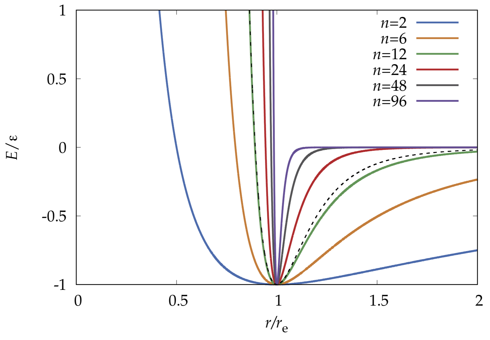
The Generalized Lennard-Jones potential for different exponents \((m, n)\) with fixed \(n = 2m\). As the exponents grow smaller, the potential flattens out and becomes softer, but as the exponents grow larger the potential becomes narrower and sharper, and approaches the hard sphere potential.

static overlapping_sphere(mu=1, [kc=1], [kh=0], [r0=0], [min=0.001], max=[10], [tol=0.001])¶

Parameters:

mu – interaction strength, represents the potential energy peak value.
kc – decay strength of long range attraction. Larger values make a shorter ranged function.
kh – Optionally add a harmonic long-range attraction, same as glj() function.
r0 – Optional harmonic rest length, only used if kh is non-zero.
min – Minimum value potential is computed for.
max – Potential cutoff values.
tol – Tolerance, defaults to 0.001.

The overlapping_sphere function implements the Overlapping Sphere, from [OFPF+17]. This is a soft sphere, from our testing, it appears too soft, probably better suited for 2D models. This potential appears to allow particles to collapse too closely, probably needs more paramater fiddling.

Note

From the equation below, we can see that there is a \(\log\) term as the short range repulsion term. The logarithm is the radial Green’s function for cylindrical (2D) geometry, however the Green’s function for 3D is the \(1/r\) function. This is possibly why Osborne has success in 2D but it’s unclear if this was used in 3D geometries.

\[\begin{split}\mathbf{F}_{ij}= \begin{cases} \mu_{ij} s_{ij}(t) \hat{\mathbf{r}}_{ij} \log \left( 1 + \frac{||\mathbf{r}_{ij}|| - s_{ij}(t)}{s_{ij}(t)} \right) ,& \text{if } ||\mathbf{r}_{ij}|| < s_{ij}(t) \\ \mu_{ij}\left(||\mathbf{r}_{ij}|| - s_{ij}(t)\right) \hat{\mathbf{r}}_{ij} \exp \left( -k_c \frac{||\mathbf{r}_{ij}|| - s_{ij}(t)}{s_{ij}(t)} \right) ,& \text{if } s_{ij}(t) \leq ||\mathbf{r}_{ij}|| \leq r_{max} \\ 0, & \text{otherwise} \\ \end{cases}\end{split}\]

Osborne refers to \(\mu_{ij}\) as a “spring constant”, this controls the size of the force, and is the potential energy peak value. \(\hat{\mathbf{r}}_{ij}\) is the unit vector from particle \(i\) center to particle \(j\) center, \(k_C\) is a parameter that defines decay of the attractive force. Larger values of \(k_C\) result in a shaper peaked attraction, and thus a shorter ranged force. \(s_{ij}(t)\) is the is the sum of the radii of the two particles.

We can plot the overlapping sphere function to get an idea of it’s behavior:

>>> import mechanica as m
>>> p = m.Potential.overlapping_sphere(mu=10, max=20)
>>> p.plot(s=2, force=True, potential=True, ymin=-10, ymax=8)

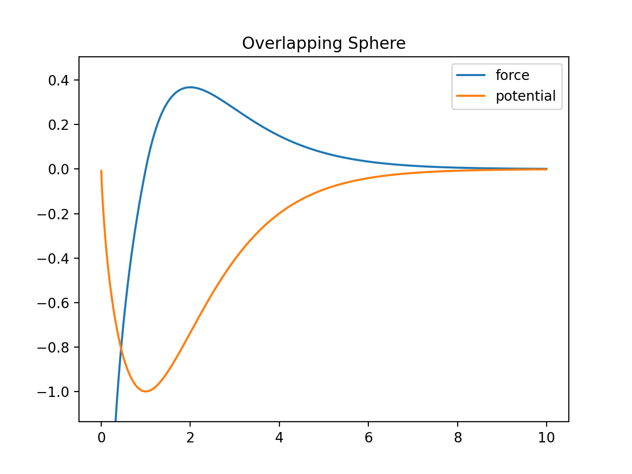
We can plot the overlapping sphere function like any other function.

static linear(k, [min], max=[10], [tol=0.001])¶

Parameters:	k – interaction strength, represents the potential energy peak value. min – Minimum value potential is computed for. max – Potential cutoff values. tol – Tolerance, defaults to 0.001.

The linear potential is the simplest one, it’s simply a potential of the form

\[U(r) = k r\]

>>> import mechanica as m
>>> p = p = m.Potential.linear(k=5, max=10)
>>> p.plot(potential=True)

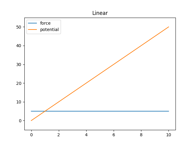
Linear potential function

Dissapative Particle Dynamics¶

Potential.dpd(alpha=1, gamma=1, sigma=1, cutoff=1)¶

Parameters:	alpha – interaction strength of the conservative force gamma – interaction strength of dissapative force sigma – strength of random force.

The dissapative particle dynamics force is the sum of the conservative, dissapative and random forces:

\[\mathbf{F}_{ij} = \mathbf{F}^C_{ij} + \mathbf{F}^D_{ij} + \mathbf{F}^R_{ij}\]

The conservative force is:

\[\mathbf{F}^C_{ij} = \alpha \left(1 - \frac{r_{ij}}{r_c}\right) \mathbf{e}_{ij}\]

The dissapative force is:

\[\mathbf{F}^D_{ij} = -\gamma \left(1 - \frac{r_{ij}}{r_c}\right)^{2}(\mathbf{e}_{ij} \cdot \mathbf{v}_{ij}) \mathbf{e}_{ij}\]

And the random force is:

\[\mathbf{F}^R_{ij} = \sigma \left(1 - \frac{r_{ij}}{r_c}\right) \xi_{ij}\Delta t^{-1/2}\mathbf{e}_{ij}\]

class DPDPotential¶: A subtype of the Potential class that adds features specific to Dissapative Particle Dynamics.