Cell Sorting
In this section, we use cell sorting as a motivating example to develop a mechanica model. We first introduce the biological phenomena, then we start our analysis by first identifying what are the key objects and processes in the biological descrioption, and how we represent these physical concepts with Mechanica objects and processes.
Cell sorting between biological cells of different types is one of the basic mechanisms creating tissue domains during develoment and wound healing and in maintaining domains in homeostasis. Cells of two different types, when dissociated and randomly mixed can spontaneously sort to reform ordered tissues. Cell sorting can generate regular patterns such as checkerboards, engulfment of one cell type by another, or other more complex patterns [Ste70].
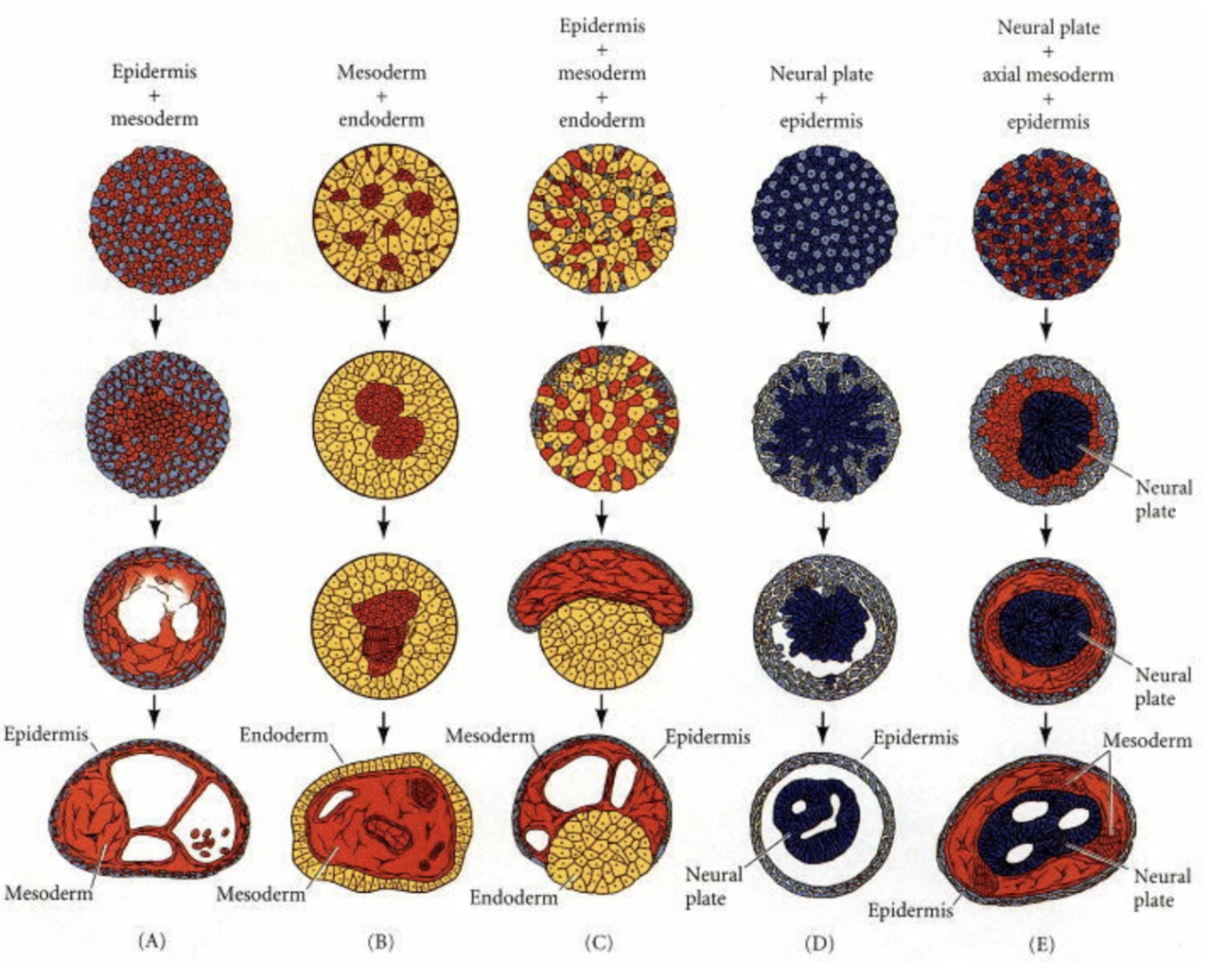
Fig. 7 A combination of cells from 3-germ layers are dissociiated and re-organize, each cell type sorts out into its own region [TH55].
Both complete and partial cell sorting (where clusters of one cell type are trapped or contained inside a closed envelope of another cell type) have been observed experimentally in vitro in embryonic cells. Cell sorting does not involve cell division nor differentiation but only spatial rearrangement of cell positions.
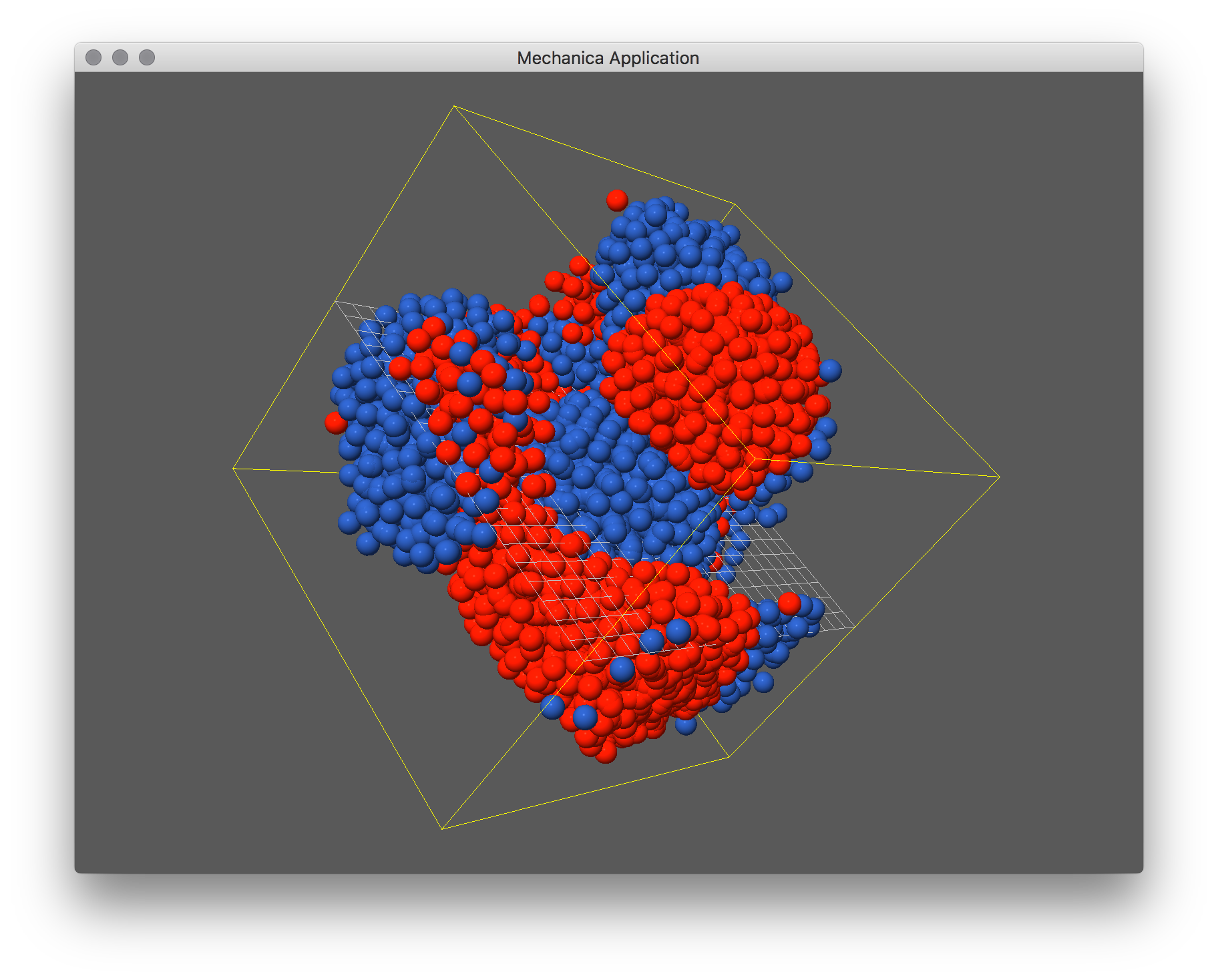
Fig. 8 A basic two-type simulation, about 25 lines of Python, as a simple extension of the two type example.
In a classic in vitro cell sorting experiment to determine relative cell adhesivities in embryonic tissues, mesenchymal cells of different types are dissociated, then randomly mixed and reaggregated. Their motility and differential adhesivities then lead them to rearrange to reestablish coherent homogenous domains with the most cohesive cell type surrounded by the less-cohesive cell types [AP72] [AA84].
Cell-sorting behavior of cell aggregates is similar to liquid surface tension, in the spontaneous separation of immiscible liquids (water vs. oil). Adhesive forces between mixed cells play a similar role in cell sorting that intermolecular attractive (cohesive) forces play in liquid surface tension. In cell sorting, the cells with the strongest highest adhesivities will be sorted to the center, while the less cohesive ones will remain outside.
Modeling and Abstraction
To develop a computational model of our biological system, we must first identify the key objects and processes of our physical system. If we look at the left side of the following figure, we can see a sheet of biogical cells. From the previous description of the cell sorting, we also know that cells move about. We know that epethelial sheets are essentially a sheet of cells that form a surface. Here we can identify our first biogical object, a cell. From the previous discussion, we know that there are more than one type of cell, so lets call our two cell types, cell type A and cell type B.
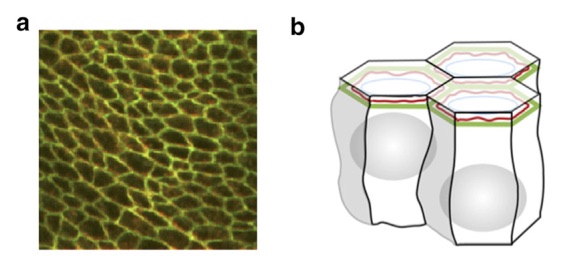
Fig. 9 On the left is a confocal microscope image of a developing Drosophila wing, where the outlines of the cells have been highlighte with a florescent protein, which binds to E-cadherin, a surface proteion involved in cell adhesion. We can represent this sheet of biological cells with a set of polygons constrained to a two dimensional surface. Taken from [FOBS14]
Example Model
We start the example just like other Mechania models:
import mechanica as m
import numpy as np

# total number of cells
A_count = 5000
B_count = 5000

# potential cutoff distance
cutoff = 3

# dimensions of universe
dim=np.array([20., 20., 20.])
center = dim / 2

# new simulator, don't load any example
m.Simulator(dim=dim, cutoff=cutoff)
We make two different cell types, A and B:
class A(m.Particle):
  mass = 1
  radius = 0.5
  dynamics = m.Overdamped


class B(m.Particle):
  mass = 1
  radius = 0.5
  dynamics = m.Overdamped
To represent the cell interactions, we create three different interacation potentials, pot_aa, pot_bb, and pot_ab. These represent the strength of interaction between cell types:
# create three potentials, for each kind of particle interaction
pot_aa = m.Potential.soft_sphere(kappa=400, epsilon=40, r0=1.5, \
                               eta=2, tol = 0.05, min=0.01, max=3)

pot_bb = m.Potential.soft_sphere(kappa=400, epsilon=40, r0=1.5, \
                               eta=2, tol = 0.05, min=0.01, max=3)

pot_ab = m.Potential.soft_sphere(kappa=400, epsilon=5, r0=1.5, \
                               eta=2, tol = 0.05, min=0.01, max=3)
And bind those potentials to our cell types:
# bind the potential with the *TYPES* of the particles
m.Universe.bind(pot_aa, A, A)
m.Universe.bind(pot_bb, B, B)
m.Universe.bind(pot_ab, A, B)
We need a random force to keep the cells moving around, this represents basically a cell motility:
# create a random force. In overdamped dynamcis, we neeed a random force to
# enable the objects to move around, otherwise they tend to get trapped
# in a potential
rforce = m.forces.random(0, 50)

# bind it just like any other force
m.bind(rforce, A)
m.bind(rforce, B)
Create the particle instances:
# create particle instances, for a total A_count + B_count cells
for p in np.random.random((A_count,3)) * 15 + 2.5:
  A(p)

for p in np.random.random((B_count,3)) * 15 + 2.5:
  B(p)
And finally run the simulation:
# run the simulator
m.Simulator.run()
The complete simulation script is here, and can be downloaded here:
Download: this example script: